library(tidyverse) library(RColorBrewer) library(circlize) library(stringr) # --- Step 1: Build communication matrix ---sent_df <- other_communications_df %>%filter(communication_type =="sent") %>%count(sender_name, recipient_name, name ="sent")received_df <- other_communications_df %>%filter(communication_type =="received") %>%count(sender_name = recipient_name, recipient_name = sender_name, name ="received")combined_df <-full_join(sent_df, received_df, by =c("sender_name", "recipient_name")) %>%mutate(across(c(sent, received), ~replace_na(., 0)),total = sent + received)comm_matrix <-xtabs(total ~ sender_name + recipient_name, data = combined_df)# --- Step 2: Assign color per entity sub-type ---type_lookup <- other_communications_df %>%select(name = sender_name, type = sender_sub_type) %>%bind_rows(other_communications_df %>%select(name = recipient_name, type = recipient_sub_type)) %>%distinct(name, .keep_all =TRUE)# Define pastel Set2 colors for each typetype_colors_palette <-brewer.pal(n =4, name ="Set2")names(type_colors_palette) <-c("Person", "Organization", "Vessel", "Location")# Map to nodes in the matrixgrid_colors <- type_colors_palette[type_lookup$type]names(grid_colors) <- type_lookup$namegrid_colors <- grid_colors[rownames(comm_matrix)]# --- Step 3: Plot chord diagram ---circos.clear()par(mar =c(4, 2, 8, 10)) # bottom, left, top, rightchordDiagram( comm_matrix,grid.col = grid_colors,transparency =0.25,annotationTrack ="grid",preAllocateTracks =list(track.height =0.1))# Add readable sector namescircos.trackPlotRegion(track.index =1,panel.fun =function(x, y) { name <-get.cell.meta.data("sector.index")circos.text(x =mean(get.cell.meta.data("xlim")),y =0,labels =str_wrap(name, 10),facing ="clockwise",niceFacing =TRUE,adj =c(0, 0.5),cex =0.6 ) },bg.border =NA)# --- Step 4: Title, subtitle ---title(main ="Chord Diagram of Communication Flows",cex.main =1.6,font.main =2,line =5)mtext("Each ribbon shows volume of sent + received messages", side =3, line =3, cex =1, col ="gray30")mtext("Note. Group subtype is excluded from this diagram", side =1, line =3, cex =0.8, col ="gray40")# --- Step 5: Custom Legend ---legend_items <-names(type_colors_palette)legend(x =1.1, y =0.85, legend = legend_items,fill = type_colors_palette,border ="gray30",bty ="n",cex =0.7,pt.cex =0.7,title ="Entity Sub-Type")
Findings
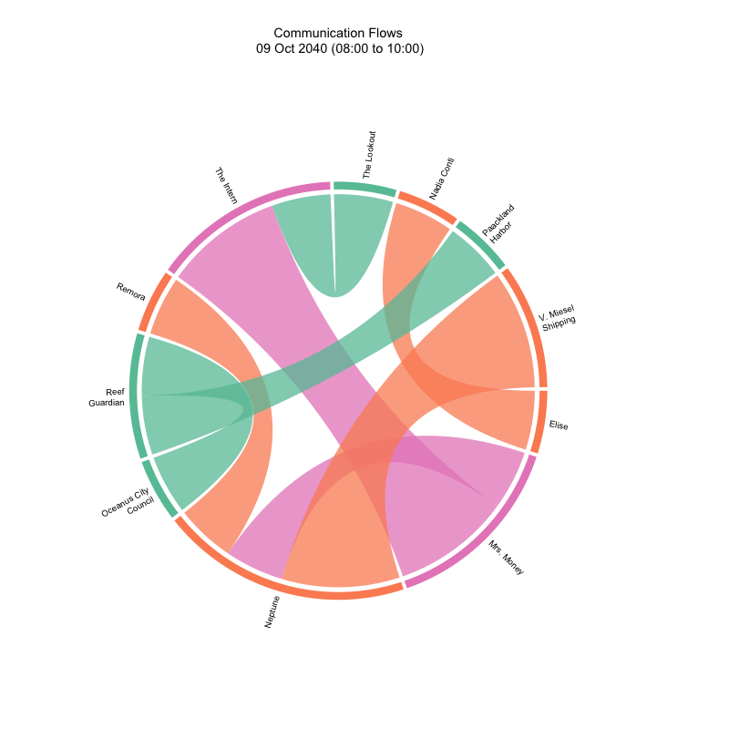
The thickness of each ribbon (chord) represents the magnitude of the relationship. A thicker ribbon represents more frequent communications (sent + received) between a sender and recipient.
Here, we have an overview of paired communicators who have higher frequencies. We also can see the links between communicators. These are the entities who communicated frequently with others that we might want to focus on:
Person: The Intern, The Lookout, Clepper Jensen, Davis, Miranda Jordan, Mrs. Money.
Organization: Oceanus City Council, Green Guardian
Vessel: Reef Guardian, Neptune, Mako, Remora
Location: Himark Habor
Group: N/A
1.2 Interactive Chord Diagram by Community
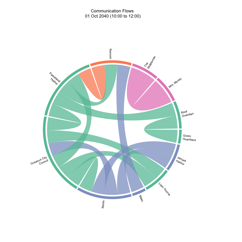
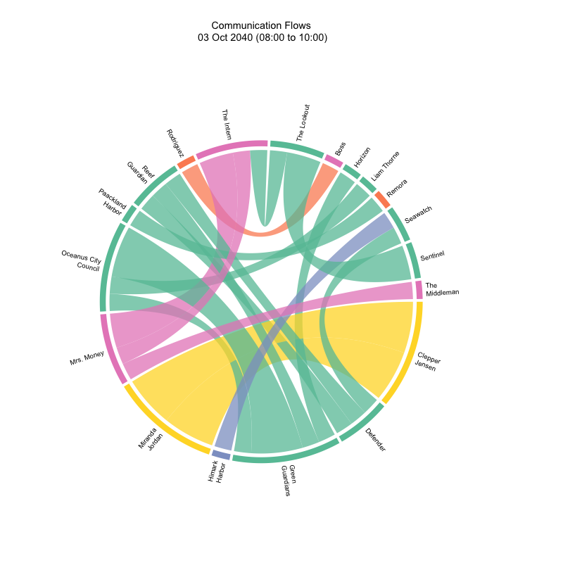
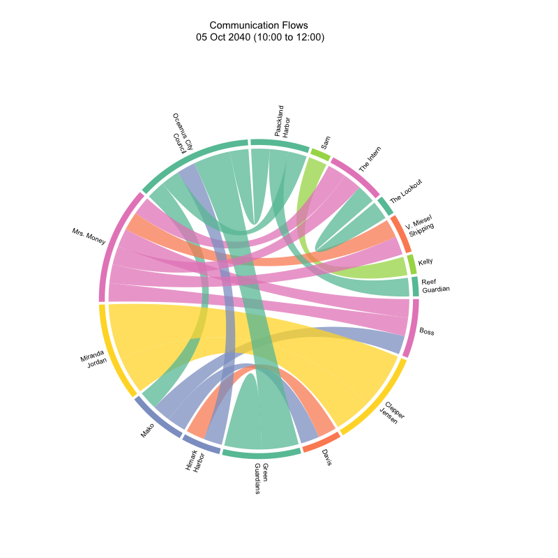
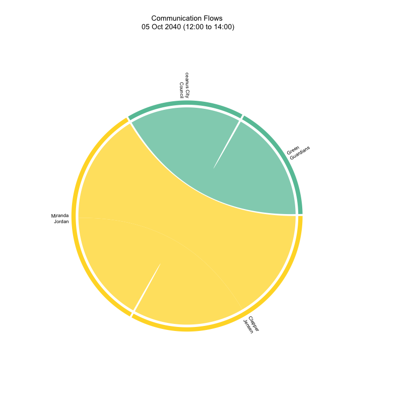
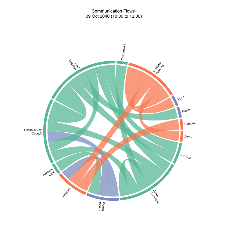
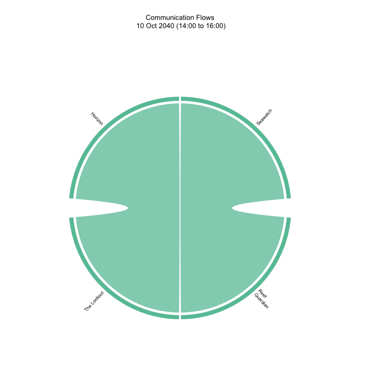
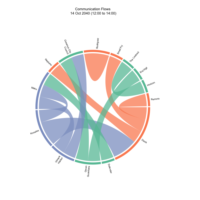
Here, the interactive chord diagram showed the correspondences among communities at every two hour intervals.
Show the code
library(circlize)library(dplyr)library(tidyr)library(RColorBrewer)library(stringr)library(lubridate)library(htmltools) # Essential for building the HTML structurelibrary(jsonlite) # For passing R data to JavaScript safely# --- 1. Data Preprocessing and Setup ---# Bin by 2-hour intervalother_communications_df <- other_communications_df %>%mutate(timestamp =as.POSIXct(timestamp)) %>%# Ensure timestamp is POSIXctmutate(timestamp_2hr =floor_date(timestamp, unit ="2 hours"))# Get all unique 2-hour time bins for the sliderall_times <-sort(unique(other_communications_df$timestamp_2hr))# Define output directory for image framesoutput_dir <-"chord_frames"dir.create(output_dir, showWarnings =FALSE) # Create the directory if it doesn't exist# Community name mapping (ensure this matches 'community_df' structure)community_name_map <-c("1"="Conservationist Group","2"="Sailor Shift","3"="Maritime","4"="Suspicious Characters","5"="Sam & Kelly","6"="Hacklee Herald")# Assuming community_df has a 'community' column that's numeric/factorif (exists("community_df") &&"community"%in%names(community_df)) { num_unique_communities <-length(unique(community_df$community)) base_colors <-brewer.pal(max(3, num_unique_communities), "Set2") # Use Set2 for pastel community_colors <-setNames( base_colors[1:num_unique_communities], # Slice to exactly the number neededas.character(sort(unique(community_df$community))) )} else {# Fallback if community_df is not defined or missing 'community' columnmessage("Warning: 'community_df' or 'community' column not found. Using default colors.") community_colors <-c("1"="#66C2A5", "2"="#FC8D62", "3"="#8DA0CB", "4"="#E78AC3","5"="#A6D854", "6"="#FFD92F", "7"="#E5C494", "8"="#B3B3B3" )}# --- 2. Generate and Save Chord Diagrams as PNGs ---# Loop through each time bin, create a plot, and save itfor (i inseq_along(all_times)) { selected_time <- all_times[i] end_time <- selected_time +hours(2) filtered_df <- other_communications_df %>%filter(timestamp_2hr == selected_time)# Prepare data for the chord diagram matrix sent_df <- filtered_df %>%filter(communication_type =="sent") %>%count(sender_name, recipient_name, name ="sent") received_df <- filtered_df %>%filter(communication_type =="received") %>%count(sender_name = recipient_name, recipient_name = sender_name, name ="received") combined_df <-full_join(sent_df, received_df, by =c("sender_name", "recipient_name")) %>%mutate(across(c(sent, received), ~replace_na(., 0)),total = sent + received)# Skip this iteration if no data for the current time sliceif (nrow(combined_df) ==0||sum(combined_df$total) ==0) {message(paste("No communications for time:", selected_time, ". Skipping frame."))next } comm_matrix <-xtabs(total ~ sender_name + recipient_name, data = combined_df)# Ensure sector_names from comm_matrix exist in community_df for color mapping sector_names <-union(rownames(comm_matrix), colnames(comm_matrix))# Filter community_df to only relevant sectors and ensure distinct entries sector_community_df <- community_df %>%filter(name %in% sector_names) %>%distinct(name, .keep_all =TRUE) %>%arrange(match(name, sector_names))# Map community colors to sector names based on 'community' column grid_colors_current_frame <-setNames( community_colors[as.character(sector_community_df$community)], sector_community_df$name )# Ensure only colors for actual sectors in the matrix are used grid_colors_current_frame <- grid_colors_current_frame[names(grid_colors_current_frame) %in% sector_names]# Open PNG device for saving the plotpng(sprintf("%s/frame_%03d.png", output_dir, i), width =800, height =800)# Clear existing circlize plot before drawing new onecircos.clear()par(mar =c(6, 2, 10, 6)) # Adjust margins as needed for title and labels# Draw the chord diagramchordDiagram( comm_matrix,grid.col = grid_colors_current_frame,transparency =0.25,annotationTrack ="grid",preAllocateTracks =list(track.height =0.1) )# Add labels to the sectorscircos.trackPlotRegion(track.index =1,panel.fun =function(x, y) { name <-get.cell.meta.data("sector.index") wrapped_name <-str_wrap(name, width =12)circos.text(x =mean(get.cell.meta.data("xlim")),y =0,labels = wrapped_name,facing ="clockwise",niceFacing =TRUE,adj =c(0, 0.5),cex =0.8 ) },bg.border =NA )# Add a main title to the plottitle(main =paste("Communication Flows\n", format(selected_time, "%d %b %Y (%H:%M"), "to", format(end_time, "%H:%M)")),cex.main =1.2,font.main =1,line =6 )dev.off() # CRITICAL: Close the PNG device to save the file}# --- 3. Build the HTML Viewer with Embedded Images and JavaScript ---# Generate HTML <img> tags for each saved frame# Filter out any frames that might have been skipped if 'next' was used# Check which frame files actually existexisting_frames <-list.files(output_dir, pattern ="^frame_\\d{3}\\.png$", full.names =TRUE)# Extract the numeric index from the filename to match with all_timesframe_indices <-as.numeric(gsub("frame_(\\d{3})\\.png", "\\1", basename(existing_frames)))# Only create image tags for the frames that were successfully generatedimage_tags <-lapply(seq_along(existing_frames), function(idx) {# The original 'i' (loop index) corresponds to the 'frame_indices' original_time_idx <- frame_indices[idx] tags$img(src = existing_frames[idx], # Use the full path herestyle =if (idx ==1) "display:block;"else"display:none;", # Show first frame by defaultclass ="chord-frame",alt =paste("Chord diagram for time slice", format(all_times[original_time_idx], "%d %b %Y %H:%M")))})# JavaScript function to update which image frame is visible# We need to map the slider value (0 to num_frames-1) to the correct time index# because some frames might be skipped, causing gaps in numerical sequence.js_script <-HTML(sprintf("<script> // Ensure the allTimes array correctly maps to the generated frames const originalAllTimes = %s; // This is the full list of all_times const generatedFrameIndices = %s; // This indicates which original_time_idx corresponds to a generated frame function updateFrame(sliderIndex) { const frames = document.querySelectorAll('.chord-frame'); frames.forEach((el, i) => { // frames[i] corresponds to existing_frames[i] from R // sliderIndex is 0-based for the slider el.style.display = (i === sliderIndex) ? 'block' : 'none'; }); // Update the time display text based on the current frame's original time const timeDisplay = document.getElementById('current-time-display'); if (timeDisplay && sliderIndex < generatedFrameIndices.length) { // Get the original time index for the currently displayed frame const actualTimeIndex = generatedFrameIndices[sliderIndex] - 1; // Convert 1-based to 0-based for originalAllTimes if (actualTimeIndex >= 0 && actualTimeIndex < originalAllTimes.length) { const selectedTime = new Date(originalAllTimes[actualTimeIndex]); const endTime = new Date(selectedTime.getTime() + 2 * 60 * 60 * 1000); // Add 2 hours in milliseconds // Format dates and times for display const formatDate = (date) => date.toLocaleDateString('en-US', { day: '2-digit', month: 'short', year: 'numeric' }); const formatTime = (date) => date.toLocaleTimeString('en-US', { hour: '2-digit', minute: '2-digit', hour12: false }); timeDisplay.innerHTML = `Day: ${formatDate(selectedTime)} | Time: ${formatTime(selectedTime)} to ${formatTime(endTime)}`; } else { timeDisplay.innerHTML = 'No data for this time slice.'; } } } // Initialize the display on page load document.addEventListener('DOMContentLoaded', () => { const slider = document.getElementById('frameSlider'); if (slider) { updateFrame(parseInt(slider.value)); // Set initial frame based on slider's default value } });</script>", jsonlite::toJSON(as.character(all_times)), jsonlite::toJSON(frame_indices))) # Pass all_times and frame_indices to JS# --- 4. Display the HTML content directly in the Quarto document ---# This is the key line to make Quarto embed the interactive viewer.browsable(tagList( js_script, # The JavaScript for interactivity tags$head( tags$style(HTML(" /* Basic styling for the image frames and slider container */ .chord-frame { width: 100%; max-width: 800px; height: auto; margin: auto; display: block; } #slider-container { text-align: center; margin: 20px auto; max-width: 800px; } .chord-title { text-align: center; font-size: 1.5em; margin-bottom: 15px; font-weight: bold; } #frameSlider { width: 80%; max-width: 700px; margin: 10px auto; display: block; } #current-time-display { font-weight: bold; margin-top: 10px; } ")) ), # Close tags$head tags$body( tags$div(class ="chord-title", "Interactive Communication Flows Over Time"), tags$div(id ="slider-container", tags$input(type ="range", min ="0", max =length(existing_frames) -1, value =0,id ="frameSlider", oninput ="updateFrame(parseInt(this.value))"), tags$p(id ="current-time-display", style ="font-weight:bold; margin-top: 10px;"), tags$p("Use the slider to view communication over time") ), tags$div(id ="chord-images-container", image_tags) # Container for all image frames ) ))
Interactive Communication Flows Over Time
Use the slider to view communication over time
1.2 Findings
We noticed some cross community direct and indirect communication occured mainly among influential nodes, suggesting collaboration. These are some sample linkages with arrows regardless of sent or received:
Community X
Node Linkages (Community X -> Community X -> Community Y)
Suspicious Characters
Mrs. Money -> Intern -> The Lookout
Liam -> Paackland Harbor -> The Middleman
Glitters Team -> Boss -> Mako
Glitters Team -> Samantha Blake -> Sailor Shifts Team
Sailor Shift
Neptune -> Elise -> Mako
Neptune -> Davis -> Mako
Remora -> Neptune -> Boss
Rodriguez -> Remora -> Mako
Remora -> Small Fry -> Mako
Davis -> Remora -> Paackland Harbor
V. Miesel Shipping -> Neptune -> Mako
Sam & Kelly
Kelly -> Sam - > The Lookout
Maritime
Mako -> Himark Harbor -> Oceanus City Council
Hacklee Herald
N/A (Only Direct Community X to X communications)
Conservationist Group
Reef Guardian -> Oceanus City Council -> Nadia
Reef Guardian -> Paackland Harbor -> Mako
Oceanus City Council -> Liam -> Nadia
We also noticed that at times, certain individuals sent messages but there were no response back. This could possibly be due to the pseudonyms being used to send or reply to the same content. For instance, there was a message from Davis to Rodriguez on 14 Oct around 1200-1400 but there was no response by Rodriguez. By looking at the content field, we then found out that he was Small Fry due to the responses he provided to Davis which was originally addressed to Rodriguez.
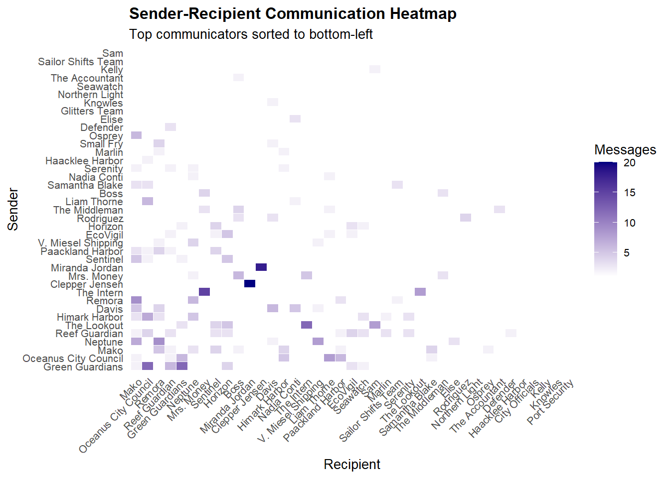
# Step 1: Count interactionsadj_df <- other_communications_df %>%count(sender_name, recipient_name, name ="count")# Step 2: Compute total sent and received countssender_order <- adj_df %>%group_by(sender_name) %>%summarise(total_sent =sum(count)) %>%arrange(desc(total_sent)) %>%pull(sender_name)recipient_order <- adj_df %>%group_by(recipient_name) %>%summarise(total_received =sum(count)) %>%arrange(desc(total_received)) %>%pull(recipient_name)# Step 3: Reorder factor levelsadj_df <- adj_df %>%mutate(sender_name =factor(sender_name, levels = sender_order),recipient_name =factor(recipient_name, levels = recipient_order) )# Step 4: Plot heatmapggplot(adj_df, aes(x = recipient_name, y = sender_name, fill = count)) +geom_tile(color ="white") +scale_fill_gradient(low ="white", high ="navyblue") +labs(title ="Sender-Recipient Communication Heatmap",subtitle ="Top communicators sorted to bottom-left",x ="Recipient",y ="Sender",fill ="Messages" ) +theme_minimal(base_size =10) +theme(axis.text.x =element_text(angle =45, hjust =1),plot.title =element_text(size =12, face ="bold"),plot.subtitle =element_text(size =10),panel.grid =element_blank() )
1.3 Findings
After extraction of the entities who communicated frequently (from the Static Chord Diagram), we tabled who they communicated with by using the heatmap. E.g. Name1 communicated with Name2.
Name 1 Subtype
Name1
Name2
Person
The Intern
The Lookout, Mrs. Money
Person
Clepper Jensen
Miranda Jordan
Person
Davis
Neptune
Person
Mrs. Money
The Intern, The Middleman, Boss
Vessel
Mako
Remora, Green Guardians, Oceanus City Council, Neptune, Reef Guardians, Himark Harbor, Davis, Sentinel, Paackland Habor, Samantha Blake, Serenity, Osprey
Vessel
Remora
Mako, Neptune, Himark Habor, Davis, Paackland Harbor, V. Miesel Shipping, Marlin, Small Fry
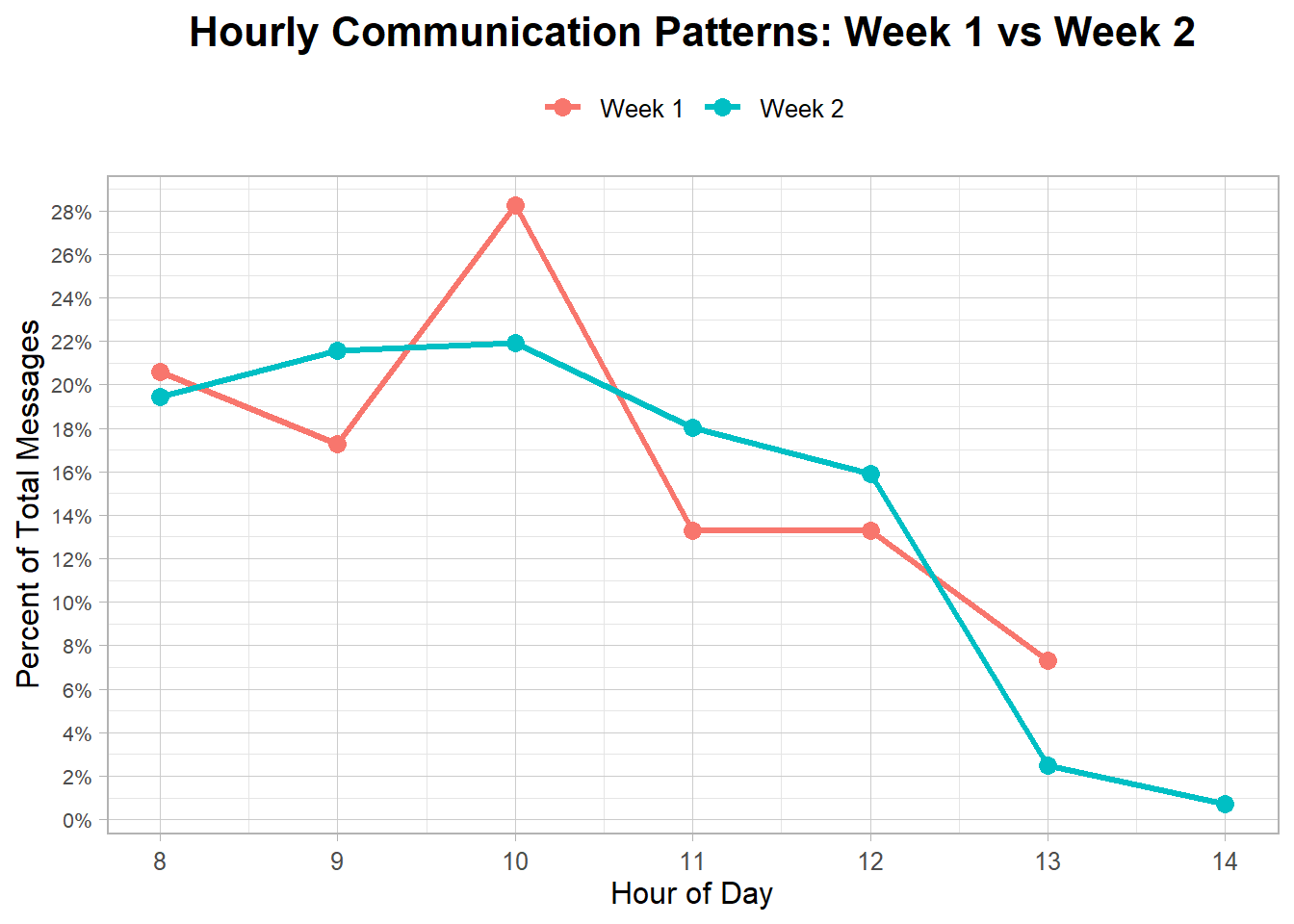
msgs <- msgs %>%mutate(week =if_else(date <=min(date) +days(6), "Week 1", "Week 2") )# Count and normalize within each weekweek_patterns <- msgs %>%count(week, hour) %>%group_by(week) %>%mutate(proportion = n /sum(n))hour_breaks <-seq(min(week_patterns$hour), max(week_patterns$hour), by =1)prop_breaks <-seq(0,ceiling(max(week_patterns$proportion) *100) /100,by =0.02)ggplot(week_patterns, aes(x = hour, y = proportion, color = week)) +geom_line(size =1.2) +geom_point(size =3) +scale_x_continuous(breaks = hour_breaks) +scale_y_continuous(breaks = prop_breaks,labels =percent_format(accuracy =1) ) +labs(title ="Hourly Communication Patterns: Week 1 vs Week 2",x ="Hour of Day",y ="Percent of Total Messages" ) +theme_light(base_size =12) +theme(plot.title =element_text(face ="bold", size =16, hjust =0.5),legend.position ="top",legend.title =element_blank(),panel.grid.major =element_line(color ="grey80"),panel.grid.minor =element_line(color ="grey90"),axis.text.x =element_text(vjust =0.5),axis.text.y =element_text(size =8) )
1.5 Findings
The visualization of hourly communication patterns reveals that message activity in Oceanus follows a pronounced daily cycle, with distinct peaks and lows across both observed weeks.
In Week 1, communication is highly concentrated in the morning hours, particularly between 8 AM and 12 PM, where a majority of the messages are exchanged.
By contrast, Week 2 shows a broader distribution of communication throughout the day, with notable increases in afternoon and evening activity.
This shift suggests that while the first week’s communications were more focused and possibly related to regular planning or operational updates, the second week’s patterns reflect heightened activity or more dynamic coordination, potentially due to emergent events or increased urgency among entities.
If two names appear as sender and recipient in the same message, they cannot belong to the same person — i.e., they’re not aliases of each other.
If two names sent a message at the exact time, they cannot belong to the same person.
For instance, if Nadia sent a message to The Accountant, they would not be the same individual. If Nadia sent a message at 10am to The Accountant and The Lookout also sent a message at 10am to The Intern, Nadia and The Lookout cannot be the same person.
Select only The Accountant, Mrs. Money, Elise: We see close timings between Mrs. Money and Elise on 8 Oct, and 10 Oct. These were on the same topic. Elise then disappears from radar on 10 Oct. She reappears as The Accountant and Mrs. Money on 11 Oct on the same topic and remains only as The Accountant till 14 Oct.
Select only Liam and The Middleman: The Middleman disappeared on 7 Oct and appeared as Liam on 8 Oct. On 11 Oct Mrs. Money asked The Middleman if anything was found by conservation vessels. On the same day, Liam reappeared and replied Elise that nothing was found by them.
Select only The Boss and Nadia: The Boss disappeared on 5 Oct and reappeared as Nadia on 8 Oct. Likely the same person.
Select only Small Fry and Rodriguez: on 2 Oct Rodriguez corresponded with Remora and Mako on meeting at the slip #14. It happened again on 14 Oct as he took on dual roles and responded to the same message with different names. Likely the same person.
Select only The Lookout and Sam: on 7 Oct Sam asked Kelly to get information on who authorized the permit. 2 minutes later, The Lookout (Kelly) responded to The Intern (Sam), that it was signed by Jensen from City Council.
Seawatch only appeared on 10 Oct but Horizon talked to Seawatch on 8 Oct. Therefore, some other entity is Seawatch before or during 8 Oct. Defender told Seawatch on 3 Oct at 8.39am that it increased its patrol and informed Seawatch to maintain vigilance. The Lookout (Seawatch) responded to Sentinel (Defender) at 8.41am that it acknowledged the need for vigilance.
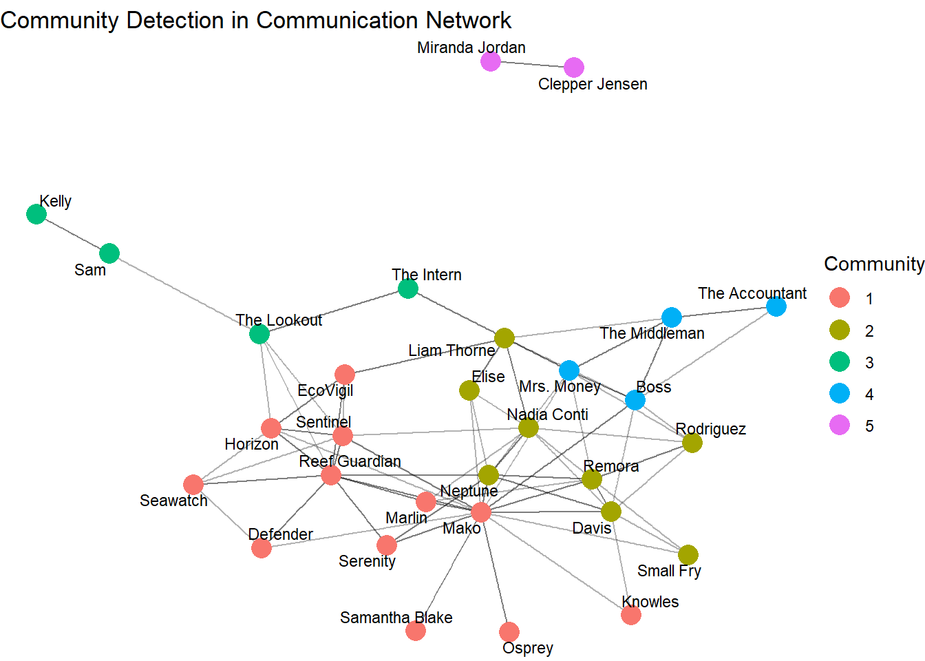
set.seed(1234)# --- STEP: Compute Centrality Measures ---g_pv <- g_pv %>%mutate(pagerank =centrality_pagerank(),degree =centrality_degree(),betweenness =centrality_betweenness(),closeness =centrality_closeness() )# Show top 10 nodes by PageRankg_pv %>%as_tibble() %>%select(name, pagerank, degree, betweenness, closeness) %>%arrange(desc(pagerank)) %>%head(10)# Visualize by Centralityggraph(g_pv, layout ="fr") +geom_edge_link(alpha =0.3) +geom_node_point(aes(size = pagerank, color =as.factor(community)), alpha =0.8) +geom_node_text(aes(label = name), repel =TRUE, size =3) +theme_void() +labs(title ="Network with PageRank Centrality",size ="PageRank", color ="Community")
2.3.1 Findings:
There were 5 closely associated groups. Community 5 (Clepper and Miranda) appeared to be segmented from the central group, due to the non-involvement from the nature of their investigative work.
From the graph, we extracted the 8 influential nodes to focus on:
Community 1: Mako
Community 2: Neptune, Remora, Nadia, Davis
Community 3: N/A as they were not very influential at global level
Community 4: Mrs. Money, Boss, The Middleman
Community 5: N/A as they were not very influential at global level
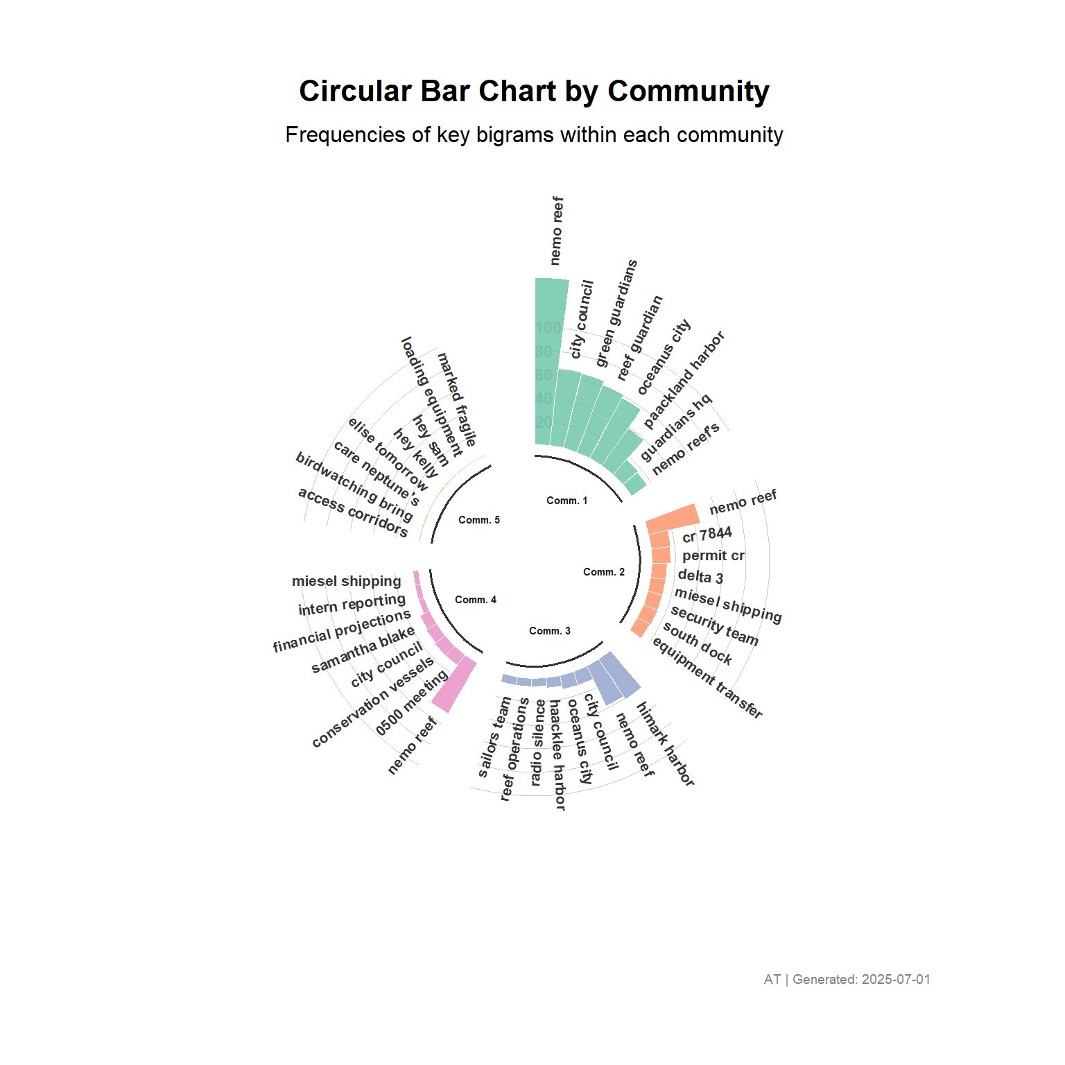
2.4 Wordclouds- Bigrams
We focused on bigrams here to get more contextual data from two instead of one word.
set.seed(1234)valid_communities <- g_pv %>%as_tibble() %>%distinct(community) %>%pull(community)bigrams <- bigrams %>%filter(community %in% valid_communities)# --- Configuration ---num_top_bigrams_per_community <-8empty_bar_count <-2# gaps btw comm.#excluded_community <- 5 # too little in community 5# --- 1. Prepare the Combined Dataset ---all_communities_data <- bigrams %>%# filter(community != excluded_community) %>%group_by(community) %>%arrange(desc(n)) %>%slice_head(n = num_top_bigrams_per_community) %>%ungroup()all_communities_data$community <-as.factor(all_communities_data$community)to_add <-data.frame(bigram =NA,n =NA,community =rep(levels(all_communities_data$community), each = empty_bar_count))plot_data <-rbind(all_communities_data, to_add) %>%arrange(community)plot_data$id <-seq_len(nrow(plot_data)) # Keep ID as numeric here# --- 2. Prepare Label Data ---label_data <- plot_datanumber_of_bar <-nrow(label_data)label_data$angle <-90-360* (label_data$id -0.5) / number_of_barlabel_data$hjust <-ifelse(label_data$angle <-90, 1, 0)label_data$angle <-ifelse(label_data$angle <-90, label_data$angle +180, label_data$angle)# --- 3. Prepare Data for Baselines (Community Dividers) ---base_data <- plot_data %>%group_by(community) %>%summarize(start =min(id, na.rm =TRUE), # Keep as numericend =max(id, na.rm =TRUE) - empty_bar_count # Keep as numeric ) %>%rowwise() %>%mutate(title_position =mean(c(start, end)) ) %>%ungroup()# --- 4. Prepare Data for Grid Lines (Optional: Value Scales) ---max_n_value <-max(plot_data$n, na.rm =TRUE)grid_lines_values <-c(20, 40, 60, 80, 100)grid_lines_values <- grid_lines_values[grid_lines_values <= max_n_value]grid_segments_data <- plot_data %>%group_by(community) %>%summarize(start_id =min(id, na.rm =TRUE), # Keep as numericend_id =max(id, na.rm =TRUE) - empty_bar_count # Keep as numeric )grid_data_final <-tibble()for(val in grid_lines_values) { temp_data <- grid_segments_data %>%mutate(y_value = val) grid_data_final <-bind_rows(grid_data_final, temp_data)}# --- Data for grid line LABELS ---grid_label_data <-data.frame(x_pos =max(plot_data$id, na.rm =TRUE) +2, # Fixed x position outside the ploty_pos = grid_lines_values,label_text =as.character(grid_lines_values))# --- 5. Make the Unified Plot ---p <-ggplot(plot_data, aes(x = id, y = n, fill = community)) +# <--- x = id (numeric)# Add background grid lines for value (e.g., 20, 40, 60, 80)geom_segment(data = grid_data_final,aes(x = start_id -0.5, y = y_value, xend = end_id +0.5, yend = y_value),inherit.aes =FALSE,color ="grey", alpha =0.8, linewidth =0.3) +# Add text showing the value of each grid line at a fixed positiongeom_text(data = grid_label_data,aes(x = x_pos, y = y_pos, label = label_text),inherit.aes =FALSE,color ="grey", size =3, angle =0, fontface ="bold", hjust =0) +# Bars for the bigrams (main plot elements)geom_bar(stat ="identity", alpha =0.8, color ="white", linewidth =0.1,width =1) +# <--- Add width=1 to remove space between bars if id is numeric# Set limits for the y-axis, providing space for labelsylim(-max_n_value *0.7, max_n_value *1.2) +theme_minimal() +theme(legend.position ="none",axis.text =element_blank(),axis.title =element_blank(),panel.grid =element_blank(),plot.margin =unit(c(1.5, 1.5, 1.5, 1.5), "cm") # Top, Right, Bottom, Left margins ) +coord_polar(start =0) +# Add bigram labelsgeom_text(data = label_data,aes(x = id, y = n +10, label = bigram, hjust = hjust), # <--- x = id (numeric)color ="black", fontface ="bold", alpha =0.8, size =2.8,angle = label_data$angle, inherit.aes =FALSE ) +# Add base lines for each community segmentgeom_segment(data = base_data,aes(x = start -0.5, y =-10, xend = end +0.5, yend =-10),colour ="black", alpha =0.8, linewidth =0.6, inherit.aes =FALSE ) +# Add community group labelsgeom_text(data = base_data,aes(x = title_position, y =-40, label =paste("Comm.", community)),colour ="black", alpha =0.9, size =2, fontface ="bold", inherit.aes =FALSE )+# --- Add the Title ---labs(title ="Circular Bar Chart by Community",subtitle ="Frequencies of key bigrams within each community", # Updated subtitlecaption =paste0("AT | Generated: ", Sys.Date()) ) +# Apply the Set2 Brewer palettescale_fill_brewer(palette ="Set2") +# --- Customize title appearance ---theme(plot.title =element_text(hjust =0.5, size =16, face ="bold", margin =margin(b =10)),plot.subtitle =element_text(hjust =0.5, size =12, margin =margin(b =10)),plot.caption =element_text(hjust =1, size =7, color ="grey50") )print(p)
2.6 Community Group Membership- People & Vessels
The topic area was gathered from the bigram wordclouds and circular bar chart. The Group Name was created based on knowledge from the Members in the group and the topic area. These are the information for the 5 segmented groups:
Suspicious (Influential Nodes: Mrs. Money, Boss, The Middleman).
We held back on the slightly less influential nodes such as: Hacklee Herald which was where Clepper Jensen worked as a journalist.
2.7 Discussion/ Interpretation:
We mainly focused on the conversations by 8 influential nodes and some related nodes:
Conservation Group (Comm.1): Samantha Blake informed Mako to stop operations on 8 and 10th Oct. Serenity is a private luxury yacht. Osprey was likely a tourism vessel looking for charter from Mako for their tourists.
Permit (Comm. 2): Neptune, Remora, Nadia, and Davis were working on Nemo Reef operation. This referred to the Music Video Production for Sailor Shift on 14 Oct.
*Pseudonym* (Comm. 3): Other than communicating among themselves, The Lookout appeared to have also externally corresponded with Sentinel, Reef Guardian and Horizon (conservation based topics), while The Intern also externally corresponded with Mrs. Money.
Suspicious (Comm. 4): The Middleman had access to Council documents. Mrs. Money had funding from sources that would not flag out to regulators for her operations. Mrs. Money was investigating V. Miesel’s structures. On 5 Oct, Boss told Mrs. Money to disguise financial trails through tourism ventures and destroy evidence of Nemo Reef operations.
Hacklee Herald (Comm. 5): Conversations between Clepper and his intern Miranda which ended on 11 Oct. Miranda mentioned an Oceanus City Council Member meeting with unmarked vessels at night.
Question 3
Question 3a)
3.1 Entities Breakdown
Core Logic:
If two names appear as sender and recipient in the same message, they cannot belong to the same person — i.e., they’re not aliases of each other.
If two names sent a message at the exact time, they cannot belong to the same person.
We created Alluvial Diagrams to chart: real_identity → observed_name → community
Real Identity from analysis -> Observed Name from data -> Community
This will probably be a drop down for each name in Shiny.
Question 3b)
We created a graph with the character’s original name, pseudonyms, and supplemented with any background information we learnt of. For instance, we learnt that Davis was a captain, or that Serenity was a private luxury yacht.Here, it is easier to determine who is using which pseudonyms by clicking on the real identity drop down panel which will then only segregate to the individual’s Real Identity, Observed Name, and Community.
Question 3c)
Understanding pseudonyms significantly reshapes our interpretation of the events in Oceanus. Without resolving aliases, the communication network appears fragmented — it may seem like dozens of separate individuals are involved. However, by mapping pseudonyms to real identities, we discover that a small number of actors are coordinating more activity than initially apparent. For example, a person using multiple pseudonyms may appear in many places at once — suggesting high influence or deception. This reveals orchestrated behavior, such as coordinated logistics, manipulation of event timelines, or masking involvement in controversial operations.
set.seed(1234)# Assume g_full includes Nadia — not g from other_communications_dfg_igraph <-as.igraph(g)# Confirm Nadia existsif (!"Nadia Conti"%in%V(g_igraph)$name) stop("Nadia Conti not found in the graph.")# Get ego subgraphnadia_ego_igraph <-make_ego_graph(g_igraph, order =1, nodes =which(V(g_igraph)$name =="Nadia Conti"), mode ="all")[[1]]# Convert to tidygraphnadia_ego_graph <-as_tbl_graph(nadia_ego_igraph)# Convert to undirected for Louvainnadia_ego_graph <- nadia_ego_graph %>%to_undirected() %>%activate(nodes) %>%mutate(community =group_louvain(),pagerank =centrality_pagerank() )# Plot Nadia's ego networkggraph(nadia_ego_graph, layout ="fr") +geom_edge_link(alpha =0.4) +geom_node_point(aes(size = pagerank, color =as.factor(community)), alpha =0.9) +geom_node_text(aes(label = name), repel =TRUE, size =3) +scale_color_brewer(palette ="Set2") +theme_void() +labs(title ="Nadia Conti’s Ego Network",subtitle ="Nodes sized by PageRank, colored by Louvain community",color ="Community",size ="PageRank" )
Note
We wanted to find out if there were sub communities within Nadia’s direct network that worked closely together.
The orange community were possibly involved in Sailor Shifts’s music video, while the green community were likely regarding ensuring compliance to authorities such as officials, the harbour and conservation team.
Nadia, Elise, and Marlin were the orange nodes that directly linked to the green nodes.
4.2 Nadia’s Sent and Received Ego Networks- VizNetwork
|communication_type |sender_id   |recipient_id         |recipient_name       |recipient_sub_type |event_id                |content                                                                                                                                                                                                                                                                                    |timestamp           |sender_name |sender_sub_type |
|:------------------|:-----------|:--------------------|:--------------------|:------------------|:-----------------------|:------------------------------------------------------------------------------------------------------------------------------------------------------------------------------------------------------------------------------------------------------------------------------------------|:-------------------|:-----------|:---------------|
|sent               |Nadia Conti |Haacklee Harbor      |Haacklee Harbor      |Location           |Event_Communication_331 |Haacklee Harbor, this is Nadia Conti. I need to cancel the special access corridor arrangements for Nemo Reef immediately. Plans have changed due to unforeseen circumstances. Destroy all related documentation. I'll contact you when we're ready to proceed with alternative locations. |2040-10-05 09:45:00 |Nadia Conti |Person          |
|sent               |Nadia Conti |Oceanus City Council |Oceanus City Council |Organization       |Event_Communication_334 |This is Nadia Conti. My cancellation was due to scheduling conflicts with our tourism development initiatives. I wasn't aware of any permit approvals. I'll submit revised documentation for alternative sustainable tourism proposals next week.                                          |2040-10-05 09:49:00 |Nadia Conti |Person          |
|sent               |Nadia Conti |Liam Thorne          |Liam Thorne          |Person             |Event_Communication_529 |Liam, Nadia here. Need your services urgently. Investigation brewing around Nemo Reef permits. Double your usual fee if you can ensure Harbor Master remains cooperative through next week. Meet at the usual place tomorrow, 10PM.                                                        |2040-10-08 08:18:00 |Nadia Conti |Person          |
|sent               |Nadia Conti |Neptune              |Neptune              |Vessel             |Event_Communication_536 |Neptune, this is Nadia. Need clarity on 'underwater foundation work' at Nemo Reef. This extends beyond our agreed scope. Meet me at the marina tomorrow at 6AM to discuss implications and additional resource requirements.                                                               |2040-10-08 08:25:00 |Nadia Conti |Person          |
|sent               |Nadia Conti |Neptune              |Neptune              |Vessel             |Event_Communication_538 |Neptune, Nadia here. Just confirming our 0600 meeting at the marina. I've reviewed the modified equipment specs with The Accountant. Please bring detailed timeline for foundation work and cost implications. We need to stay under radar.                                                |2040-10-08 08:30:00 |Nadia Conti |Person          |
|sent               |Nadia Conti |Marlin               |Marlin               |Vessel             |Event_Communication_584 |Marlin, Nadia here. I understand you're inquiring about eastern shoal routes. Those are temporary diversions due to equipment transport needs. I'll have Davis provide the necessary documentation tonight. Nothing to be concerned about.                                                 |2040-10-08 11:23:00 |Nadia Conti |Person          |
|sent               |Nadia Conti |Liam Thorne          |Liam Thorne          |Person             |Event_Communication_795 |Liam, Nadia here. Redirect all remaining operations from southwest immediately. Move equipment to our secondary location. I'll handle EcoVigil through proper channels. Meet me at the usual place at 2100 hours with updated documentation.                                               |2040-10-12 08:44:00 |Nadia Conti |Person          |
|sent               |Nadia Conti |V. Miesel Shipping   |V. Miesel Shipping   |Organization       |Event_Communication_847 |This is Nadia. Documentation for permit #CR-7844 is complete. Meeting The Middleman at 2100 to handle final details. Recommend accelerating timeline due to EcoVigil's ROV approval. Shifting operations from southwest immediately. Will update after meeting.                            |2040-10-12 11:19:00 |Nadia Conti |Person          |
[1] "--- Nadia's Received Communications ---"
|communication_type |sender_id            |sender_name          |sender_sub_type |recipient_id |event_id                |content                                                                                                                                                                                                                                                                                                  |timestamp           |recipient_name |recipient_sub_type |
|:------------------|:--------------------|:--------------------|:---------------|:------------|:-----------------------|:--------------------------------------------------------------------------------------------------------------------------------------------------------------------------------------------------------------------------------------------------------------------------------------------------------|:-------------------|:--------------|:------------------|
|received           |Haacklee Harbor      |Haacklee Harbor      |Location        |Nadia Conti  |Event_Communication_330 |Haacklee Harbor to Nadia Conti. Following your visit yesterday regarding the Nemo Reef event logistics, we've prepared the necessary documentation. Harbor staff is ready to facilitate the special access corridor arrangements as discussed. Please confirm timeline for implementation.               |2040-10-05 09:44:00 |Nadia Conti    |Person             |
|received           |Oceanus City Council |Oceanus City Council |Organization    |Nadia Conti  |Event_Communication_333 |Ms. Conti, this is Oceanus City Council. We need clarification regarding your canceled Nemo Reef event arrangements at Haacklee Harbor. Please explain your documentation destruction request immediately. This relates to our newly expedited permit approvals.                                         |2040-10-05 09:48:00 |Nadia Conti    |Person             |
|received           |Sailor Shifts Team   |Sailor Shifts Team   |Organization    |Nadia Conti  |Event_Communication_520 |Hi Nadia, this is the Sailor Shifts Team. Received your message about permit assistance - thank you! We urgently need to discuss tomorrow's staffing requirements. Can you confirm how many additional crew members we should bring for the setup?                                                       |2040-10-07 11:57:00 |Nadia Conti    |Person             |
|received           |Davis                |Davis                |Person          |Nadia Conti  |Event_Communication_521 |Davis, Nadia here. Let's meet at 7PM at the marina office to review documentation. I've been working with alternative channels for permits. Bring all shipping manifests - we'll need to create a clean paper trail immediately.                                                                         |2040-10-07 12:00:00 |Nadia Conti    |Person             |
|received           |Elise                |Elise                |Person          |Nadia Conti  |Event_Communication_528 |Nadia, Elise here. Meeting at Nemo Reef 0500 tomorrow to establish payment protocols. Sam uncovered V. Miesel shipping lanes overlapping with Mako by 40%. Neptune mentioned 'underwater foundation work' - outside our original scope. Need your assessment.                                            |2040-10-08 08:15:00 |Nadia Conti    |Person             |
|received           |Liam Thorne          |Liam Thorne          |Person          |Nadia Conti  |Event_Communication_535 |Nadia, Liam here. Meeting confirmed for tomorrow at 10PM. I've redirected Harbor Master's attention and implemented new patrol schedules that work in our favor. Council suspects nothing about Nemo Reef. Bring payment as discussed.                                                                   |2040-10-08 08:24:00 |Nadia Conti    |Person             |
|received           |Neptune              |Neptune              |Vessel          |Nadia Conti  |Event_Communication_537 |Neptune to Nadia. I'm aware of the foundation work concerns. We're delivering the additional heavy equipment today as requested. Will meet you at 0600 as planned to discuss resource adjustments and review modified equipment specifications that Elise has approved funding for.                      |2040-10-08 08:27:00 |Nadia Conti    |Person             |
|received           |Davis                |Davis                |Person          |Nadia Conti  |Event_Communication_582 |Nadia, Davis here. I'll be at the marina office at 7PM with all shipping manifests. Could you bring copies of permit #CR-7844? Marlin's asking about unusual vessel routes near eastern shoals - might need to address this.                                                                             |2040-10-08 11:21:00 |Nadia Conti    |Person             |
|received           |Davis                |Davis                |Person          |Nadia Conti  |Event_Communication_585 |Davis, Marlin here again. Nadia mentioned you'd provide documentation about those eastern shoal diversions tonight. Just checking if that's still coming through. Need to understand these new patterns while my vessel's being repaired.                                                                |2040-10-08 11:26:00 |Nadia Conti    |Person             |
|received           |Elise                |Elise                |Person          |Nadia Conti  |Event_Communication_601 |Nadia, Elise here. Situation escalating. Permanent underwater construction confirmed at Nemo Reef. Sam reports concrete forms suggesting structures beyond equipment installation. Need urgent clarification on real scope and V. Miesel's involvement before tomorrow's meeting. Prepare contingencies. |2040-10-09 08:54:00 |Nadia Conti    |Person             |
[1] "--- Nadia's Full Communication Timeline (Combined) ---"
|communication_type |sender_id            |recipient_id         |recipient_name       |recipient_sub_type |event_id                |content                                                                                                                                                                                                                                                                                    |timestamp           |sender_name          |sender_sub_type |communicating_pair_sorted        |
|:------------------|:--------------------|:--------------------|:--------------------|:------------------|:-----------------------|:------------------------------------------------------------------------------------------------------------------------------------------------------------------------------------------------------------------------------------------------------------------------------------------|:-------------------|:--------------------|:---------------|:--------------------------------|
|received           |Haacklee Harbor      |Nadia Conti          |Nadia Conti          |Person             |Event_Communication_330 |Haacklee Harbor to Nadia Conti. Following your visit yesterday regarding the Nemo Reef event logistics, we've prepared the necessary documentation. Harbor staff is ready to facilitate the special access corridor arrangements as discussed. Please confirm timeline for implementation. |2040-10-05 09:44:00 |Haacklee Harbor      |Location        |Haacklee Harbor_Nadia Conti      |
|sent               |Nadia Conti          |Haacklee Harbor      |Haacklee Harbor      |Location           |Event_Communication_331 |Haacklee Harbor, this is Nadia Conti. I need to cancel the special access corridor arrangements for Nemo Reef immediately. Plans have changed due to unforeseen circumstances. Destroy all related documentation. I'll contact you when we're ready to proceed with alternative locations. |2040-10-05 09:45:00 |Nadia Conti          |Person          |Haacklee Harbor_Nadia Conti      |
|received           |Oceanus City Council |Nadia Conti          |Nadia Conti          |Person             |Event_Communication_333 |Ms. Conti, this is Oceanus City Council. We need clarification regarding your canceled Nemo Reef event arrangements at Haacklee Harbor. Please explain your documentation destruction request immediately. This relates to our newly expedited permit approvals.                           |2040-10-05 09:48:00 |Oceanus City Council |Organization    |Nadia Conti_Oceanus City Council |
|sent               |Nadia Conti          |Oceanus City Council |Oceanus City Council |Organization       |Event_Communication_334 |This is Nadia Conti. My cancellation was due to scheduling conflicts with our tourism development initiatives. I wasn't aware of any permit approvals. I'll submit revised documentation for alternative sustainable tourism proposals next week.                                          |2040-10-05 09:49:00 |Nadia Conti          |Person          |Nadia Conti_Oceanus City Council |
|received           |Sailor Shifts Team   |Nadia Conti          |Nadia Conti          |Person             |Event_Communication_520 |Hi Nadia, this is the Sailor Shifts Team. Received your message about permit assistance - thank you! We urgently need to discuss tomorrow's staffing requirements. Can you confirm how many additional crew members we should bring for the setup?                                         |2040-10-07 11:57:00 |Sailor Shifts Team   |Organization    |Nadia Conti_Sailor Shifts Team   |
|received           |Davis                |Nadia Conti          |Nadia Conti          |Person             |Event_Communication_521 |Davis, Nadia here. Let's meet at 7PM at the marina office to review documentation. I've been working with alternative channels for permits. Bring all shipping manifests - we'll need to create a clean paper trail immediately.                                                           |2040-10-07 12:00:00 |Davis                |Person          |Davis_Nadia Conti                |
|received           |Elise                |Nadia Conti          |Nadia Conti          |Person             |Event_Communication_528 |Nadia, Elise here. Meeting at Nemo Reef 0500 tomorrow to establish payment protocols. Sam uncovered V. Miesel shipping lanes overlapping with Mako by 40%. Neptune mentioned 'underwater foundation work' - outside our original scope. Need your assessment.                              |2040-10-08 08:15:00 |Elise                |Person          |Elise_Nadia Conti                |
|sent               |Nadia Conti          |Liam Thorne          |Liam Thorne          |Person             |Event_Communication_529 |Liam, Nadia here. Need your services urgently. Investigation brewing around Nemo Reef permits. Double your usual fee if you can ensure Harbor Master remains cooperative through next week. Meet at the usual place tomorrow, 10PM.                                                        |2040-10-08 08:18:00 |Nadia Conti          |Person          |Liam Thorne_Nadia Conti          |
|received           |Liam Thorne          |Nadia Conti          |Nadia Conti          |Person             |Event_Communication_535 |Nadia, Liam here. Meeting confirmed for tomorrow at 10PM. I've redirected Harbor Master's attention and implemented new patrol schedules that work in our favor. Council suspects nothing about Nemo Reef. Bring payment as discussed.                                                     |2040-10-08 08:24:00 |Liam Thorne          |Person          |Liam Thorne_Nadia Conti          |
|sent               |Nadia Conti          |Neptune              |Neptune              |Vessel             |Event_Communication_536 |Neptune, this is Nadia. Need clarity on 'underwater foundation work' at Nemo Reef. This extends beyond our agreed scope. Meet me at the marina tomorrow at 6AM to discuss implications and additional resource requirements.                                                               |2040-10-08 08:25:00 |Nadia Conti          |Person          |Nadia Conti_Neptune              |
[1] "--- Checking: Number of nodes and edges in Nadia's Ego Network Graph ---"
# --- 2. Clean and Prepare Nodes ---mc3_nodes_cleaned <- mc3_nodes_raw %>%mutate(id =as.character(id)) %>%filter(!is.na(id)) %>%distinct(id, .keep_all =TRUE) %>%# Rename 'type' to 'supertype' to reduce confusion with communication typerename(supertype = type) %>%# Select only columns that are needed and are consistently presentselect(id, name, sub_type, content, timestamp) # Keep timestamp as character for now# --- 3. Clean and Prepare Edges ---# Rename 'type' in edges to 'edge_type' to avoid conflict with node 'supertype'mc3_edges_cleaned <- mc3_edges_raw %>%rename(from_id = source,to_id = target,edge_type = type) %>%# Renamed 'type' to 'edge_type'mutate(across(c(from_id, to_id), as.character)) %>%# Filter out any edges where from_id or to_id are not in cleaned nodesfilter(from_id %in% mc3_nodes_cleaned$id, to_id %in% mc3_nodes_cleaned$id)# --- 4. Identify Nadia Conti's ID and Sub_type ---nadia_info <- mc3_nodes_cleaned %>%filter(name =="Nadia Conti") %>%select(id, sub_type) # Corrected: Select sub_type here, not supertypenadia_id <- nadia_info %>%pull(id)nadia_sub_type <- nadia_info %>%pull(sub_type) # New variable for Nadia's sub_typeif (length(nadia_id) ==0) {stop("Nadia Conti not found in the nodes data. Please check the 'name' column or the ID.")} elseif (length(nadia_id) >1) {warning("Multiple entries found for Nadia Conti. Using the first one.") nadia_id <- nadia_id[1] nadia_sub_type <- nadia_sub_type[1] # Ensure sub_type is also taken for the first one}print(paste("Nadia Conti's ID:", nadia_id))print(paste("Nadia Conti's Sub_type:", nadia_sub_type))# --- 5. Extract Nadia's Sent Communications ---# Logic: Nadia (source) --sent--> Event_Communication (target) --received--> Recipient (target)nadia_sent_communications <- mc3_edges_cleaned %>%filter(from_id == nadia_id, edge_type =="sent") %>%# Join with nodes to get content and timestamp of the Event_Communication nodeleft_join(mc3_nodes_cleaned %>%select(id, content, timestamp),by =c("to_id"="id")) %>%rename(event_id = to_id, event_content = content, event_timestamp = timestamp) %>%# Now, find the recipient of this communication eventleft_join(mc3_edges_cleaned %>%filter(edge_type =="received") %>%select(event_id_match = from_id, recipient_id = to_id),by =c("event_id"="event_id_match")) %>%# Join with nodes to get the recipient's name AND sub_typeleft_join(mc3_nodes_cleaned %>%select(id, name, sub_type), # Select sub_type hereby =c("recipient_id"="id")) %>%rename(recipient_name = name, recipient_sub_type = sub_type) %>%# Rename sub_type# Select and rename final columns for sent communicationsselect(communication_type = edge_type, # This will be "sent"sender_id = from_id, recipient_id, recipient_name, recipient_sub_type, # Include in final select event_id,content = event_content,timestamp = event_timestamp # Timestamp is still character here ) %>%mutate(sender_name =!!nadia_id, # Explicitly set sender_name to Nadia's ID/name using !!sender_sub_type =!!nadia_sub_type # Assign Nadia's sub_type as a constant value using !! )print("--- Nadia's Sent Communications ---")print(kable(head(nadia_sent_communications, 10), format ="markdown", align ="l"))# --- 6. Extract Nadia's Received Communications ---# Logic: Sender (source) --sent--> Event_Communication (target) --received--> Nadia (target)nadia_received_communications <- mc3_edges_cleaned %>%filter(to_id == nadia_id, edge_type =="received") %>%# The source of this edge is the Event_Communication noderename(event_id = from_id) %>%# Join with nodes to get content and timestamp of the Event_Communication nodeleft_join(mc3_nodes_cleaned %>%select(id, content, timestamp),by =c("event_id"="id")) %>%rename(event_content = content, event_timestamp = timestamp) %>%# Now, find the original sender of this communication eventleft_join(mc3_edges_cleaned %>%filter(edge_type =="sent") %>%select(event_id_match = to_id, sender_id = from_id),by =c("event_id"="event_id_match")) %>%# Join with nodes to get the sender's name AND sub_typeleft_join(mc3_nodes_cleaned %>%select(id, name, sub_type), # Select sub_type hereby =c("sender_id"="id")) %>%rename(sender_name = name, sender_sub_type = sub_type) %>%# Rename sub_type# Select and rename final columns for received communicationsselect(communication_type = edge_type, # This will be "received" sender_id, sender_name, sender_sub_type, # Include in final selectrecipient_id = to_id, event_id,content = event_content,timestamp = event_timestamp ) %>%mutate(recipient_name =!!nadia_id, # Explicitly set recipient_name to Nadia's ID/name using !!recipient_sub_type =!!nadia_sub_type # Assign Nadia's sub_type as a constant value using !! )print("--- Nadia's Received Communications ---")print(kable(head(nadia_received_communications, 10), format ="markdown", align ="l"))# --- 7. Combine Sent and Received Communications for Full Timeline ---nadia_full_communications_timeline <-bind_rows( nadia_sent_communications, nadia_received_communications) %>%arrange(timestamp) %>%# CRITICAL FIX: Explicitly convert timestamp to POSIXct after bind_rows# Use as.POSIXct with the observed format stringmutate(timestamp =as.POSIXct(timestamp, format ="%Y-%m-%d %H:%M:%S")) %>%# NEW: Create a sorted communicating pair for consistent coloringrowwise() %>%# Process row by rowmutate(communicating_pair_sorted =paste(sort(c(sender_name, recipient_name)), collapse ="_")) %>%ungroup() # Return to normal data frame operationsprint("--- Nadia's Full Communication Timeline (Combined) ---")print(kable(head(nadia_full_communications_timeline, 10), format ="markdown", align ="l"))# --- 8. Prepare Data for Ego Network Visualization (Direct Person-to-Person/Entity) ---# Build nodes and edges directly from nadia_full_communications_timeline,# focusing on direct sender-recipient connections.# Nodes for the ego network graph: Collect all unique sender and recipient IDsall_ego_person_entity_ids <- nadia_full_communications_timeline %>%select(id = sender_id) %>%bind_rows(nadia_full_communications_timeline %>%select(id = recipient_id)) %>%distinct(id) %>%filter(!is.na(id)) # Ensure no NA IDs# Filter mc3_nodes_cleaned to get attributes for these person/entity nodesego_nodes_for_graph <- mc3_nodes_cleaned %>%filter(id %in% all_ego_person_entity_ids$id) %>%filter(!is.na(id)) %>%# Ensure no NA IDs in nodes for graph# Add attributes for visualizationmutate(is_nadia =ifelse(id == nadia_id, TRUE, FALSE),# Create a new column for legend grouping that includes Nadia as a distinct categorynode_legend_group =ifelse(is_nadia, "Nadia Conti", sub_type),node_size =ifelse(is_nadia, 20, 18), # Further increased node sizes: Nadia 20, others 10display_name =ifelse(is_nadia, "Nadia Conti", name) # Use actual name for others ) %>%filter(!is.na(sub_type)) # Ensure nodes have a sub_type for consistent plotting# Calculate communication counts for each node for hover textnode_comm_summary <- nadia_full_communications_timeline %>%group_by(id = sender_id) %>%summarise(sent_count =n(), .groups ='drop') %>%full_join(nadia_full_communications_timeline %>%group_by(id = recipient_id) %>%summarise(received_count =n(), .groups ='drop'),by ="id") %>%mutate(sent_count =replace_na(sent_count, 0),received_count =replace_na(received_count, 0) )# Join communication summary and create hover text for nodesego_nodes_for_graph <- ego_nodes_for_graph %>%left_join(node_comm_summary, by ="id") %>%mutate(hover_text =paste("Name:", display_name, "<br>","Type:", node_legend_group, "<br>","Sent Communications:", sent_count, "<br>","Received Communications:", received_count ) )# Edges for the ego network graph: Direct Sender -> Recipient edges# Aggregate to count occurrences for edge thicknessego_edges_for_graph <- nadia_full_communications_timeline %>%# Group by sender, recipient, their names, and communication type to count interactionsgroup_by(from = sender_id, to = recipient_id, sender_name, recipient_name, communication_type) %>%summarise(count_of_comm =n(), # Number of times this specific communication happenedcontent_sample =paste(head(content, 1), collapse ="; "), # Sample contenttimestamp_min =min(timestamp, na.rm =TRUE),timestamp_max =max(timestamp, na.rm =TRUE),.groups ='drop' ) %>%# Add the 'nadia_role_in_comm' column for coloring based on Nadia's perspectivemutate(nadia_role_in_comm =case_when( from == nadia_id & communication_type =="sent"~"Nadia Sent", to == nadia_id & communication_type =="received"~"Nadia Received",TRUE~"Other Communication"# For communications not directly involving Nadia as sender/recipient ) ) %>%# Ensure 'from' and 'to' are character and non-NAmutate(from =as.character(from),to =as.character(to) ) %>%filter(!is.na(from) &!is.na(to)) %>%# Filter out edges where 'from' or 'to' IDs are NOT in the final ego_nodes_for_graphfilter(from %in% ego_nodes_for_graph$id, to %in% ego_nodes_for_graph$id) %>%# Create hover text for edgesmutate(hover_text =paste("From:", sender_name, "<br>","To:", recipient_name, "<br>","Type:", communication_type, "<br>","Count:", count_of_comm, "<br>","First:", format(timestamp_min, "%Y-%m-%d %H:%M:%S"), "<br>","Last:", format(timestamp_max, "%Y-%m-%d %H:%M:%S"), "<br>","Content Sample:", content_sample ) )# Create the tbl_graph object for the ego networknadia_ego_network_graph <-tbl_graph(nodes = ego_nodes_for_graph, edges = ego_edges_for_graph, directed =TRUE)print("--- Checking: Number of nodes and edges in Nadia's Ego Network Graph ---")print(paste("Nodes:", gorder(nadia_ego_network_graph), "Edges:", gsize(nadia_ego_network_graph)))print("---------------------------------------------------------------------")
4.2.2 Nadia’s Sent and Received Ego Networks
4.2.2.1 Sent Communications Network
Show the code
# Define custom colors for node types (reusing from previous code)node_legend_colors_plot <-c("Person"="#88CCEE", # Blue"Vessel"="#D55E00", # Orange"Organization"="#117733", # Green"Location"="#AA4499", # Purple"Nadia Conti"="red"# Special color for Nadia)# Define custom shapes for node subtypesnode_legend_shapes_plot <-c("Person"="dot", # Circle for visNetwork"Vessel"="triangle","Organization"="square","Location"="diamond","Nadia Conti"="star"# Star shape for Nadia in visNetwork)# Separate the edges into two sets: Nadia Sent and Nadia Receivededges_sent <- ego_edges_for_graph %>%filter(nadia_role_in_comm =="Nadia Sent")edges_received <- ego_edges_for_graph %>%filter(nadia_role_in_comm =="Nadia Received")# Function to build visNetwork plot for a given edge setbuild_visnetwork_plot <-function(edge_df, title_label) {# Prepare nodes from edge list node_ids <-unique(c(edge_df$from, edge_df$to)) nodes <- ego_nodes_for_graph %>%filter(id %in% node_ids) %>%mutate(label =ifelse(display_name =="Nadia Conti", "", display_name),title =paste0("<b>", display_name, "</b><br>","Type: ", node_legend_group, "<br>","Sent: ", sent_count, "<br>","Received: ", received_count ),group =ifelse(display_name =="Nadia Conti", "Nadia Conti", node_legend_group) ) %>%select(id, label, title, group, value = node_size)# Prepare edges with arrow and tooltip edges <- edge_df %>%filter(!is.na(from) &!is.na(to)) %>%mutate(arrows ="to",title =paste0("<b>From:</b> ", sender_name, "<br>","<b>To:</b> ", recipient_name, "<br>","<b>Type:</b> ", communication_type, "<br>","<b>Count:</b> ", count_of_comm, "<br>","<b>First:</b> ", format(timestamp_min, "%Y-%m-%d %H:%M:%S"), "<br>","<b>Last:</b> ", format(timestamp_max, "%Y-%m-%d %H:%M:%S"), "<br>","<b>Content Sample:</b><br><div style='max-width:300px;white-space:normal;'>", content_sample, "</div>" ) ) %>%select(from, to, arrows, title, width = count_of_comm)# Create visNetworkvisNetwork(nodes, edges, width ="100%", height ="600px") %>%visEdges(smooth =FALSE, arrows =list(to =list(enabled =TRUE, scaleFactor =1.5))) %>%visOptions(highlightNearest =TRUE, nodesIdSelection =TRUE) %>%visIgraphLayout(layout ="layout_with_fr") %>%visNodes(font =list(size =14)) %>%visGroups(groupname ="Person", color = node_legend_colors_plot[["Person"]], shape = node_legend_shapes_plot[["Person"]]) %>%visGroups(groupname ="Vessel", color = node_legend_colors_plot[["Vessel"]], shape = node_legend_shapes_plot[["Vessel"]]) %>%visGroups(groupname ="Organization", color = node_legend_colors_plot[["Organization"]], shape = node_legend_shapes_plot[["Organization"]]) %>%visGroups(groupname ="Location", color = node_legend_colors_plot[["Location"]], shape = node_legend_shapes_plot[["Location"]]) %>%visGroups(groupname ="Nadia Conti", color = node_legend_colors_plot[["Nadia Conti"]], shape = node_legend_shapes_plot[["Nadia Conti"]]) %>%visLegend(addNodes = legend_df,ncol =2,position ="left",main ="Entity (Sub)Types",useGroups =FALSE) %>%visLayout(randomSeed =123) %>% visNetwork::visExport() %>% visNetwork::visPhysics(enabled =TRUE) %>% visNetwork::visInteraction(navigationButtons =TRUE) %>% visNetwork::visEvents(stabilizationIterationsDone ="function () {this.setOptions({physics:false});}")}# Build and show visNetwork plotsbuild_visnetwork_plot(edges_sent, "Nadia Sent Ego Network")
4.2.2.2 Received Communications Network
Show the code
build_visnetwork_plot(edges_received, "Nadia Received Ego Network")
4.2.3 Findings
We then wanted to find more about the correspondences. The first graph illustrated Nadia’s sent communications and the second graph were her received communications. Hover over nodes to see the sent or received count from the perspective of the entity. Hover over arrowheads to see the number, direction, count, first and last correspondence time, type of sent or received, and content of one communication. Nadia sent only 8 but received 18 communications (possibly indicative of using a pseudonym):
Sent more direct communications to Liam (2) and Neptune (2), relative to others.
Received more from Davis (5), Elise (3), and Liam (2), relative to others.
The next step would be to find out the suspicious characters/ activities.
4.3 Nadia’s Ego Network: 3-hops degree centrality
To uncover more details, we designed n-hops degree centrality here. We input 3 hops to hover over the nodes and look into the communications in a wider network. 3-hop exposes overlapping communites (Nadia communicating with someone who coordinates between groups). The “bridges” may show their value in 3-hops. It also increases the change of detecting complete or near complete cliques. We understand that should there be requirements for details, we could look into n-hops and more.
Show the code
# --- Define event and relationship subtypes (optional, for filtering or labeling) ---event_subtypes <-c("Communication", "Monitoring", "VesselMovement", "Assessment","Collaborate", "Endorsement", "TourActivity", "TransponderPing","Harbor Report", "Fishing", "Criticize")relationship_subtypes <-c("Coordinates", "AccessPermission", "Operates", "Colleagues","Suspicious", "Reports", "Jurisdiction", "Unfriendly", "Friends")# --- Define node colors and shapes by type or key sub-type ---node_legend_colors_plot <-c("Person"="#88CCEE","Vessel"="#D55E00","Organization"="#117733","Location"="#AA4499","Group"="#CC79A7","Event"="#DDCC77","Relationship"="#AF8DC3")node_legend_shapes_plot <-c("Person"="dot","Vessel"="triangle","Organization"="square","Location"="diamond","Group"="circle","Event"="star","Relationship"="square")STYLES <-list(node_label_dark ="black",font_family ="Roboto Condensed")# ---- 2. Define function to extract ego subgraph ----extract_ego_subgraph <-function(center_node ="Nadia Conti", hops =3) {# Construct igraph object g <-graph_from_data_frame(d = mc3_edges_final %>%select(from = from_id, to = to_id),vertices = mc3_nodes_final %>%select(id) %>%distinct() %>%rename(name = id),directed =TRUE )# Extract ego network ego_graph <-make_ego_graph(g, order = hops, nodes = center_node, mode ="all")[[1]] node_ids <-V(ego_graph)$name edge_df <-as_data_frame(ego_graph, what ="edges")# Prepare node metadata for visNetwork ego_nodes <- mc3_nodes_final %>%filter(id %in% node_ids) %>%mutate(label =ifelse(is.na(name), id, name),tooltip_extra =case_when( type =="Event"& sub_type =="Communication"~ content, type =="Event"& sub_type =="Monitoring"~ findings, type =="Event"& sub_type =="VesselMovement"~ destination, type =="Event"& sub_type =="Assessment"~ results, type =="Relationship"& sub_type =="Coordinates"~ coordination_type, type =="Relationship"& sub_type =="Operates"~ operational_role, type =="Relationship"& sub_type =="Jurisdiction"~ jurisdiction_type,TRUE~NA_character_ ),title =paste0("<b>", label, "</b><br>","Type: ", type, "<br>","Sub-type: ", sub_type, "<br>",ifelse(!is.na(tooltip_extra), paste0("<br><b>Details:</b> ", tooltip_extra), "") ),group =case_when( sub_type %in%names(node_legend_colors_plot) ~ sub_type, type %in%names(node_legend_colors_plot) ~ type,TRUE~"Other" ) ) %>%select(id, label, group, title) %>%distinct(id, .keep_all =TRUE)list(nodes = ego_nodes, edges = edge_df)}# ---- 3. Extract Nadia Conti's 3-hop ego network ----ego_data <-extract_ego_subgraph("Nadia Conti", hops =3)nodes <- ego_data$nodesedges <- ego_data$edges# (Optional) Save outputnadia_ego_nodes_2hop <- nodesnadia_ego_edges_2hop <- edges# ---- 4. Build visNetwork plot ----net <-visNetwork(nodes, edges, width ="100%", height ="600px") %>%visEdges(arrows =list(to =list(enabled =TRUE, scaleFactor =1.5))) %>%visOptions(highlightNearest =TRUE, nodesIdSelection =TRUE) %>%visIgraphLayout(layout ="layout_with_fr") %>%visNodes(font =list(size =14,color = STYLES$node_label_dark,face = STYLES$font_family,vadjust =-15 ))# ---- 5. Apply color/shape for known groups ----used_groups <-intersect(unique(nodes$group), names(node_legend_colors_plot))for (group_name in used_groups) { net <- net %>%visGroups(groupname = group_name,color = node_legend_colors_plot[[group_name]],shape = node_legend_shapes_plot[[group_name]] )}# ---- 6. Add legend dynamically ----legend_df <- tibble::tibble(label = used_groups,shape = node_legend_shapes_plot[used_groups],color = node_legend_colors_plot[used_groups]) %>%distinct(label, .keep_all =TRUE)net <- net %>%visLegend(addNodes = legend_df,ncol =2,position ="left",main ="Entity (Sub)Types",useGroups =FALSE)# ---- 7. Render the network ----net
4.3.1 Findings
Nodes from 1-hop: Nadia, Davis, Elise, Haacklee Habor, Liam, Marlin, Neptune, Oceanus City Council, Remora, Rodriguez, Sailor Shifts Team, Sentinel, V. Miesel Shipping.
Additional nodes from 3-hop: Conservation vessels, EcoVigil, Sam, The Accountant, Mako, Nemo Reef.
We would then use these 3-hop nodes to drill in deeper to find suspicious relationships between nodes.
Elise, EcoVigil, Elise, Davis, Liam, Mako, Neptune, Sam, Remora, Rodriguez, Sailor Shifts Team, Sentinel, The Accountant, Oceanus City Council, V. Miesel Shipping possibly found something suspicious or were involved in something suspicious.
4.4.2 Plotted Timeline (3-hop)- Only suspicious communications
These are the suspicious communications extracted from 4.4.1.
There were certain questions we posted to ourselves and came out with the answers.
4.5.1 The Community and Ego Network:
Question and Answer Analysis
Question
Answer
Who were Nadia’s direct communication contacts (1-hop degree centrality)? Are any of them known to be suspicious or involved in illicit activities?
From the thicker width in the Ego network, it appeared that Nadia often communicated with Liam, Elise, and Davis.
Liam appeared to be The Middleman within Nadia’s direct community from the Louvain Community Network.
From the filtered table on suspicious relationships, Elise, Liam, EcoVigil, Sentinel, Oceanus City Council, and V. Miesel Shipping were noted to have suspicious relationships.
Their conversations were the area of focus to uncover their roles, relationships and identities.
Were there any other ‘Event’ or ‘Relationship’ nodes directly connected to Nadia in this communication network that hinted at suspicious people/ activities?
Based on information from question 2, Rodriguez was previously involved in mining activities that affected the environment. ‘Mining’ as a topic and his conversations would be tracked.
4.5.2 The Communication Timeline and Content:
In the nadia_full_communications_timeline table, the actual content of her direct two-way communications were investigated over the course of 9 days. There were certain suspicious entities, keywords, coded language, or unusual topics detected that were suspicious. We have tabled out the segmented suspicious and non-suspicious entities for investigation and elimination.
Likely conservation area which was picked by the characters for illicit activities.
331, 943
Permit #CR-7844
Item
Likely a permit to show tourism activity as a cover for suspicious activities. Rodriguez is likely linked to vessels Mako, Neptune, and Remora operating under this permit with a tourism facade.
582, 847, 805
EcoVigil
Vessel
EcoVigil will likely affect Nadia’s operations when they use their ROV. Nadia recommended to V. Miesel to accelerate the planned operation. They were likely working for different sides.
753, 847
Suspicious Entity
Sub Type
Community
Rationale
Event ID
Haacklee Harbor
Location
2
Nadia’s communication to Haacklee Harbor is suspicious when she wanted the documents destroyed and the special corridor to Nemo Reef cancelled.
331
Liam aka The Middleman
Person
2
Nadia wanted him to double his usual fee to ensure Harbor Master remains cooperative. Identity revealed through:
529, 795, 847
Davis
Person
1
Nadia told him to create a clean paper trail. She will provide permits.
521
Elise aka Mrs. Money
Person
1
Nadia warned Elise that conservation vessels might complicate their operation. Identity revealed through:
708, 528, 538, 677
Rodriguez aka Small Fry
Person
1
Linked to Mako, which is operating under a permit with a tourism facade.
805
Remora
Vessel
1
Remora reported a tourism facade to Nadia and planned underwater lighting placements in Nemo Reef while monitoring conservation vessels.
943
Neptune
Vessel
1
Nadia told Neptune to stay under the radar.
538
V. Miesel HQ
Organisation
1
Organisation was aware of the suspicious permit and The Middleman.
846, 847
Sailor Shifts Team aka Glitters Team
Organisation
1
Nadia provided crew members for the setup related to the permit.
520
Non Suspicious Entity
Sub Type
Community
Rationale
Event ID
Oceanus City Council
Organisation
2
Oceanus City Council as a whole is not suspicious as an organisation as Liam stated this organisation suspected nothing.
535
Sentinel
Vessel
2
Sentinel Vessel suspected ulterior motives as the water quality was fine.
677
Marlin
Vessel
2
Marlin inquired about unusual vessel routes near eastern shoals, Nadia and Davis might need to address this.
584
4.6 Querying Keywords
Based on our knowledge, we decided to connect to external information. We used knowledge from Nadia’s current network and communication with keyword search of our queries.
There were overlaps as the blue permit also included the red NR-1045 permit and green CR-7844 permit.
Show the code
library(reactable)library(dplyr)library(stringr)library(readr) # Used for read_lines# 1. Prepare data from the text provideddata_text <-"Date & Time | Event Description------------|---------------------------------------------------------------------------------------------------------------2 Oct (12:16pm) | Rodriguez was from the Sailor Shifts Team.5 Oct (10:54am) | Jensen from City Council approved Nemo Reef permit.6 Oct (9:57am) | Remora told Sailor Shifts Team that Nadia got Commissioner Torres to sign off the permit.6 Oct (10:45am) | Mako acknowledged NR-1045 permit to Nemo Reef.6 Oct (12:33pm) | Mako was lead vessel to Neptune and Remora as authorised by V. Miesel Shipping.7 Oct (9:40am) | Mako was operating under permit NR-1045 for conservation research.8 Oct (10:24am) | Mako was operating under V. Miesel's special marine research permit CR-7844 approved by Oceanus City Council.8 Oct (10:30am) | Mako informed Remora that both of them were operating under permit CR-7844 and have a 5 day deadline.8 Oct (10:40am) | Remora was approved by Paackland Harbor to operate with extended hours under permit NR-1045.9 Oct (11:53am) | Mako requesed for additional crew from v Miesel Shipping for the 24hr operations over next 5 days.11 Oct (6:00am) | Nemo Reef closure mandated by Oceanus City Council.11 Oct (8:57am) | All research permits must be submitted within 72 hours.11 Oct (10:05am) | V. Miesel Shipping informed Remora that 30% of her crew to be reassigned to Neptune.12 Oct (10:01am) | Davis as Captain oversaw crew reallocation.12 Oct (11:19am) | Nadia secured documentation for CR-7844.12 Oct (12:52pm) | Harbor closure for 3 days from 13 Oct 06:00."# Parse the data into a data frame# Use read_lines to handle the multi-line stringdata_lines <-read_lines(data_text)# Remove the header separator line and any empty linesdata_lines <- data_lines[!grepl("^---|===", data_lines) & data_lines !=""]# The first non-separator line is the headercol_names_raw <-str_split(data_lines[1], "\\|")[[1]]col_names <-str_trim(col_names_raw)# The rest are data rowsdata_content <- data_lines[-1]# Create data frame by splitting lines and putting into a tibbledf <-tibble(line = data_content) %>%mutate(`Date & Time`=str_trim(str_extract(line, "^[^|]+")),`Event Description`=str_trim(str_extract(line, "(?<=\\|).+$")) ) %>%select(`Date & Time`, `Event Description`) # Ensure correct column order and names# 2. Create the reactable table with desired featuresreactable( df,filterable =TRUE, # Enable column-specific filters (from the tutorial)searchable =TRUE, # Enable global search box (from the tutorial)paginationType ="numbers", # Display page numbers (corrected from "pages")defaultPageSize =5, # Show 5 rows per pageshowPageSizeOptions =TRUE, # Allow users to change page sizepageSizeOptions =c(5, 10, 15, 20, 50), # Options for page sizesstriped =TRUE, # Add alternating row colors (from the tutorial)highlight =TRUE, # Highlight row on hover (from the tutorial)columns =list(`Date & Time`=colDef(name ="Date & Time",minWidth =120, # Adjust width to fit contentalign ="left" ),`Event Description`=colDef(name ="Event Description",minWidth =500, # Ensure enough width for event descriptionsalign ="left" ) ),# Apply a custom theme for better aesthetics (inspired by the tutorial)theme =reactableTheme(borderColor ="#dfe2e5",stripedColor ="#f6f8fa",highlightColor ="#f0f5f9",cellPadding ="8px 12px",style =list(fontFamily ="Verdana, Geneva, sans-serif", fontSize ="14px"),headerStyle =list("&.rt-th:hover"=list(backgroundColor ="#e0e6eb"),fontSize ="15px",fontWeight =600,color ="#333", # Darker header text for contrastbackground ="#f7f7f7"# Slightly grey background for header ),rowSelectedStyle =list(backgroundColor ="#e6f2ff", "&:hover"=list(backgroundColor ="#e6f2ff")),# Styles for search/filter inputs (from tutorial's theme example)searchInputStyle =list(width ="100%", margin ="5px 0", padding ="5px"),filterInputStyle =list(width ="100%", margin ="2px 0", padding ="4px") ))
Since there were little communications on 13 Oct, we looked into other word queries.
Using information obtained from question 2 and 4, we had in mind certain keywords to query for.
4.6.2 Plotted Timeline (Word Query: Music Video Related)
Which vessel was the suspicious permit #CR-7844 prepared for?
(See 4.6.1.1)
From question 2 and 4, we know this is V. Miesel’s Marine Research Permit, and prepared for Mako (lead vessel), Neptune, and Remora.
What suspicious activity was performed at Nemo Reef? Which day was it?
(See 4.6.2)
14 Oct 2040 for a music video production.
Why is underwater lighting placement needed at Nemo Reef?
(See 4.6.2)
For a music video production.
What were the expedited approvals and secretive logistics?
(See 4.6.1 and 4.6.2)
Permits for Nemo Reef through NR-1045 and CR-788 were expedited. The secretive logistics were the crates and equipment on the vessels for the music video production.
Who were the high-level Oceanus officials, Sailor Shift’s team, local influential families, and local conservationist group?
(Various Ids)
Oceanus Officials: Commissioner Blake, Commissioner Torres, Council Knowles, The Middleman, Jensen, Liam Thorne
Sailor Shift’s Team: Boss, Council Knowles, Davis, Glitters Team, Liam Thorne, Mako, Mrs. Money, Nadia, Neptune, Remora, Rodriguez, Sam, Samantha Blake, Small Fry, The Accountant, The Intern, The Middleman
Local Influential Families: Council Knowles, V. Miesel Shipping
Local Conservationist Group: Defender, EcoVigil, Green Guardians, Horizon, Kelly, Reef Guardians, Seawatch, Sentinel, The Lookout
Was the music video production activity legal?
(Id 979)
There was no environmental damage or mining involved in the music production. However, an environmental assessment was not conducted prior. Clepper may assess that his suspicions about Nadia Conti’s illicit activity may not be straightforward and could depend on whether an assessment was mandatory before commercial activities.