To build this prototype module, we adopted a structured visual analytics approach, starting from data ingestion to visual storytelling. The knowledge graph provided in Mini-Challenge 3 was first cleaned, transformed, and modeled using tidygraph. Communication patterns, relationships, and anomalies were then extracted through modular analysis and visualized using both static (ggplot2, ggraph) and interactive (plotly, visNetwork) tools.
The overall methodology consists of the following stages:
Data Preparation We loaded and flattened the JSON-based knowledge graph, extracted nodes and edges, cleaned missing values, and validated the network structure for compatibility with tidygraph. Each entity was classified by type and sub-type to enable filtering and targeted analysis.
Modular Task Execution Each of the four investigative tasks was assigned to team member, allowing parallel and comparison development:
Temporal trends were analyzed by aggregating communication timestamps by hour and date.
Entity relationships were explored through network graph layouts and centrality measures.
Anomaly detection used Z-score normalization on daily message counts.
Suspicious activity was investigated through person-to-person messaging analysis.
Prototype Development All modules were translated into reactive components suitable for a Shiny application. Input widgets such as selectInput(), dateRangeInput(), and checkboxGroupInput() allow user-driven filtering, while outputs include plotlyOutput() and visNetworkOutput() for dynamic and exploratory analysis.
Design and Storyboarding A UI storyboard was drafted to guide the layout of the final Shiny app, ensuring usability and clarity. Each module was built to function independently but integrate smoothly into the full application.
1.0 Installing packages
We will use the code chunk below uses p_load() of pacman package to check if packages are installed in the computer. If they are, then they will be launched into R. Though it is not added here in pacman due to conflicts, networkD3, highcharter, leaflet, conflicted will also be added on Shiny.
It contains graph data, where nodes can be accessed via nodes and edges via links. This dataset had many columns but we filtered the relevant data during wrangling.
2.1 Defining common variables
We will also set some values for consistency throughout all graphs.
List of 5
 $ directed  : logi TRUE
 $ multigraph: logi FALSE
 $ graph     :List of 4
  ..$ mode        : chr "static"
  ..$ edge_default: Named list()
  ..$ node_default: Named list()
  ..$ name        : chr "VAST_MC3_Knowledge_Graph"
 $ nodes     :'data.frame': 1159 obs. of  31 variables:
  ..$ type             : chr [1:1159] "Entity" "Entity" "Entity" "Entity" ...
  ..$ label            : chr [1:1159] "Sam" "Kelly" "Nadia Conti" "Elise" ...
  ..$ name             : chr [1:1159] "Sam" "Kelly" "Nadia Conti" "Elise" ...
  ..$ sub_type         : chr [1:1159] "Person" "Person" "Person" "Person" ...
  ..$ id               : chr [1:1159] "Sam" "Kelly" "Nadia Conti" "Elise" ...
  ..$ timestamp        : chr [1:1159] NA NA NA NA ...
  ..$ monitoring_type  : chr [1:1159] NA NA NA NA ...
  ..$ findings         : chr [1:1159] NA NA NA NA ...
  ..$ content          : chr [1:1159] NA NA NA NA ...
  ..$ assessment_type  : chr [1:1159] NA NA NA NA ...
  ..$ results          : chr [1:1159] NA NA NA NA ...
  ..$ movement_type    : chr [1:1159] NA NA NA NA ...
  ..$ destination      : chr [1:1159] NA NA NA NA ...
  ..$ enforcement_type : chr [1:1159] NA NA NA NA ...
  ..$ outcome          : chr [1:1159] NA NA NA NA ...
  ..$ activity_type    : chr [1:1159] NA NA NA NA ...
  ..$ participants     : int [1:1159] NA NA NA NA NA NA NA NA NA NA ...
  ..$ thing_collected  :'data.frame':   1159 obs. of  2 variables:
  .. ..$ type: chr [1:1159] NA NA NA NA ...
  .. ..$ name: chr [1:1159] NA NA NA NA ...
  ..$ reference        : chr [1:1159] NA NA NA NA ...
  ..$ date             : chr [1:1159] NA NA NA NA ...
  ..$ time             : chr [1:1159] NA NA NA NA ...
  ..$ friendship_type  : chr [1:1159] NA NA NA NA ...
  ..$ permission_type  : chr [1:1159] NA NA NA NA ...
  ..$ start_date       : chr [1:1159] NA NA NA NA ...
  ..$ end_date         : chr [1:1159] NA NA NA NA ...
  ..$ report_type      : chr [1:1159] NA NA NA NA ...
  ..$ submission_date  : chr [1:1159] NA NA NA NA ...
  ..$ jurisdiction_type: chr [1:1159] NA NA NA NA ...
  ..$ authority_level  : chr [1:1159] NA NA NA NA ...
  ..$ coordination_type: chr [1:1159] NA NA NA NA ...
  ..$ operational_role : chr [1:1159] NA NA NA NA ...
 $ edges     :'data.frame': 3226 obs. of  5 variables:
  ..$ id         : chr [1:3226] "2" "3" "5" "3013" ...
  ..$ is_inferred: logi [1:3226] TRUE FALSE TRUE TRUE TRUE TRUE ...
  ..$ source     : chr [1:3226] "Sam" "Sam" "Sam" "Sam" ...
  ..$ target     : chr [1:3226] "Relationship_Suspicious_217" "Event_Communication_370" "Event_Assessment_600" "Relationship_Colleagues_430" ...
  ..$ type       : chr [1:3226] NA "sent" NA NA ...
2.3 Extracting the edges and nodes tables
Next, as_tibble() of tibble package package is used to extract the nodes and links tibble data frames from mc3 tibble dataframe into two separate tibble dataframes called mc3_nodes_raw and mc3_edges_raw respectively.
In the code chunk below, ExpCatViz() of SmartEDA package is used to reveal the frequency distribution of all categorical fields in mc3_nodes tibble dataframe.
Show the code
library(shiny)library(ggplot2)# Run ExpCatViz once at the top to avoid recomputingExpCatViz(data=mc3_nodes_raw,col="navyblue")
[[1]]
[[2]]
[[3]]
[[4]]
[[5]]
[[6]]
[[7]]
[[8]]
[[9]]
[[10]]
[[11]]
[[12]]
[[13]]
[[14]]
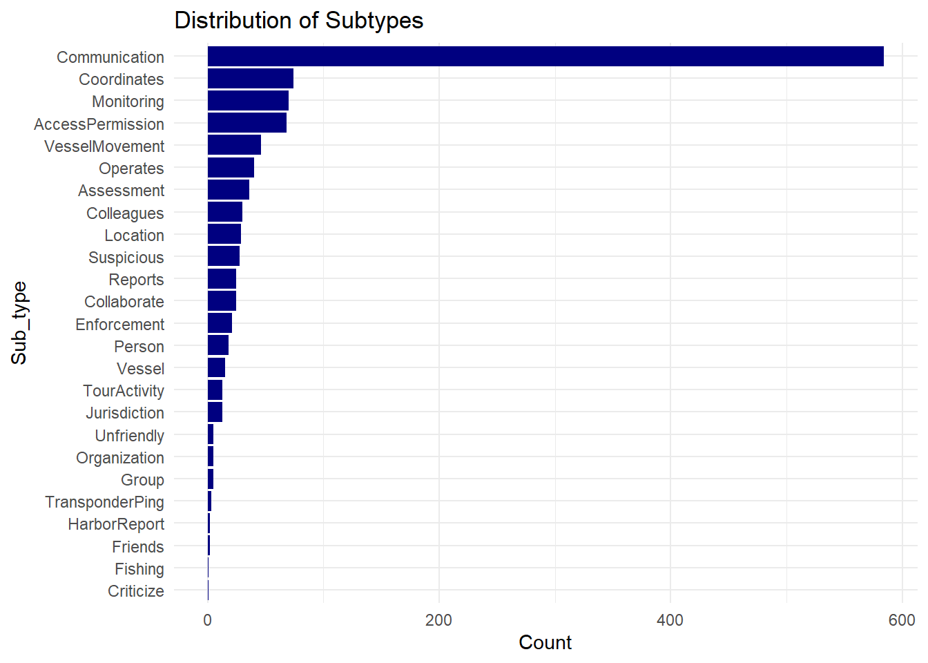
Code chunk below uses ggplot2 functions to reveal the frequency distribution of sub_type field of mc3_nodes_raw.
Show the code
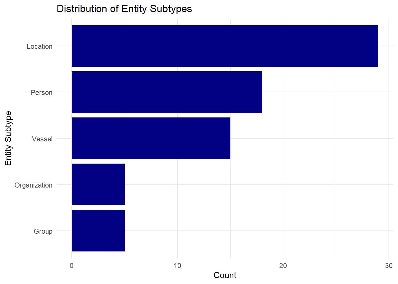
# Step 1: Count and reordermc3_nodes_ordered <- mc3_nodes_raw %>%count(sub_type) %>%arrange((n)) %>%mutate(sub_type =factor(sub_type, levels = sub_type))# Step 2: Plot with navy bars, sorted, and horizontalggplot(mc3_nodes_ordered, aes(x = sub_type, y = n)) +geom_col(fill ="navy") +coord_flip() +labs(x ="Sub_type", y ="Count",title ="Distribution of Subtypes") +theme_minimal()
In the code chunk below, the Entity subtypes are filtered.
We will use the EDA findings to determine data to focus on or eliminate. From the bar charts and the original data on mc3_nodes_raw, it was observed that:
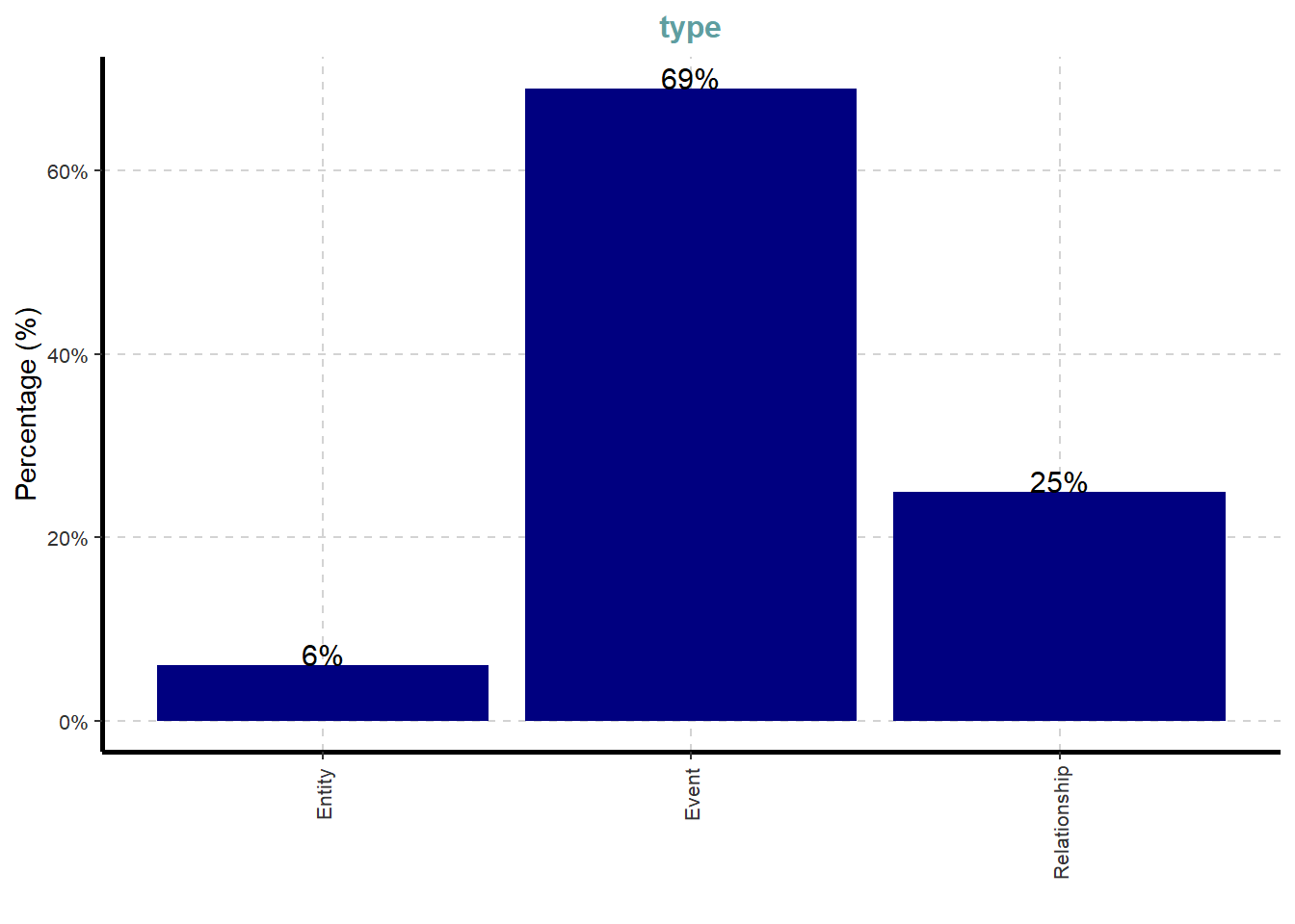
Nodes were one of three types (Entity, Event, Relationship), where each of these types have their sub_types. Majority were of event type, followed by relationship, and entity.
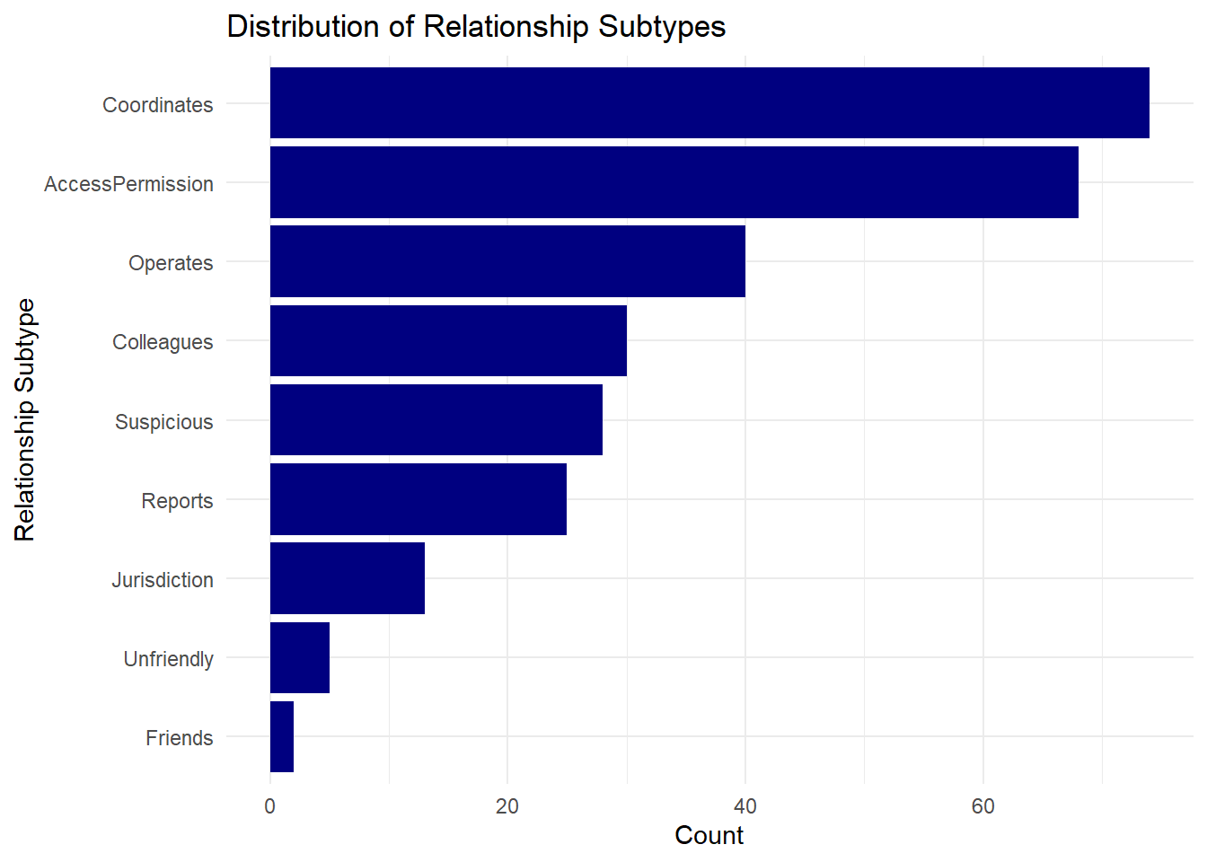
There were 25 subtypes. Communications made up the bulk of the sub_type for Events. Coordinates made up the bulk of the sub_type for Relationship. The additional node sub_types not mentioned in the VAST 2025 MC3 Data Description under Node Attributes were: fishing, communication and coordinates.
Observations of EDA from Event types:
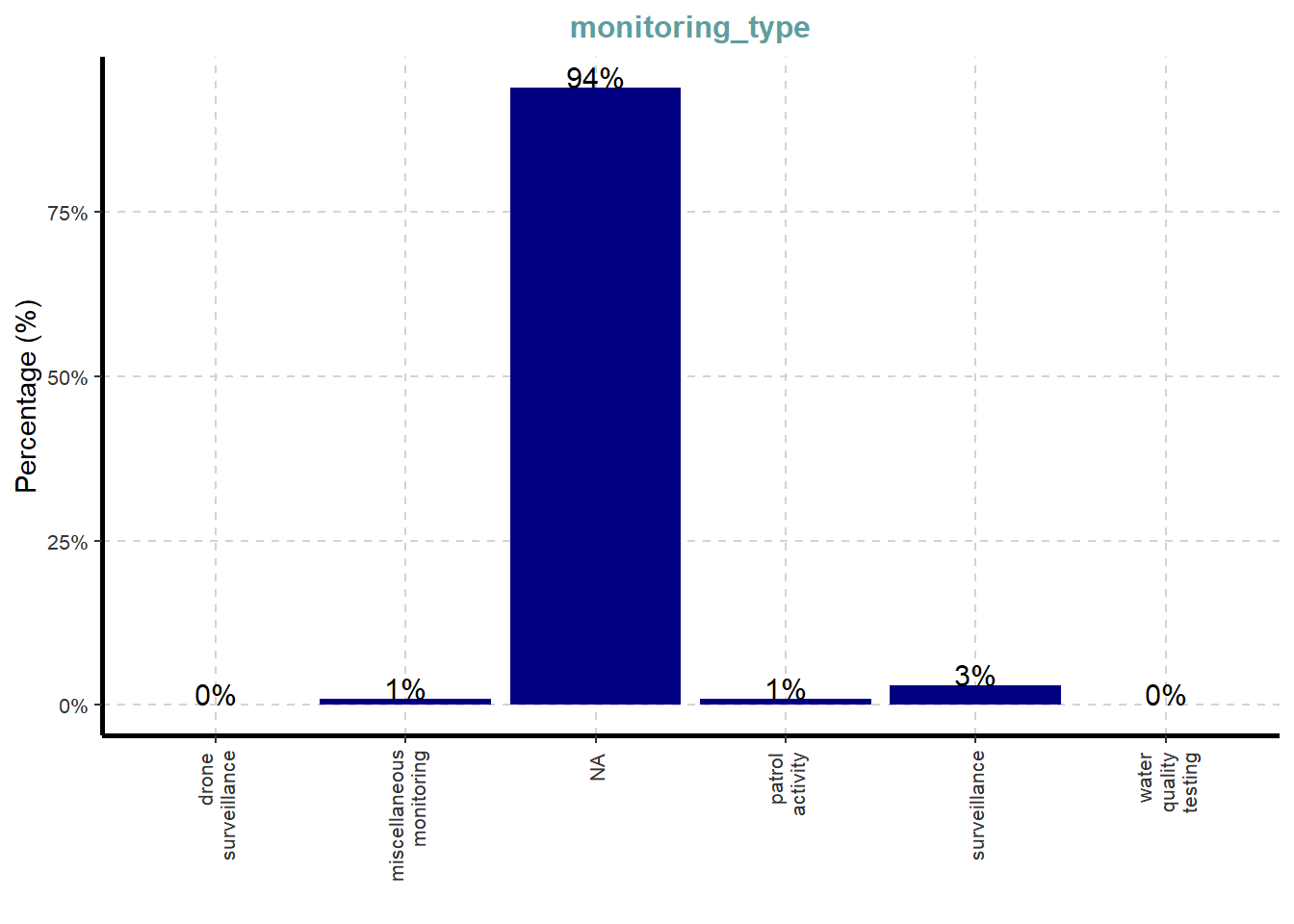
Findings field were filled when there were monitoring_type.
Content refers to radio communication content.
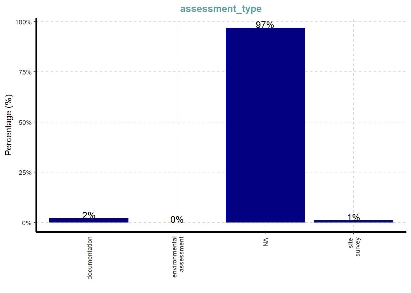
Results field were filled when there were assessment_type performed.
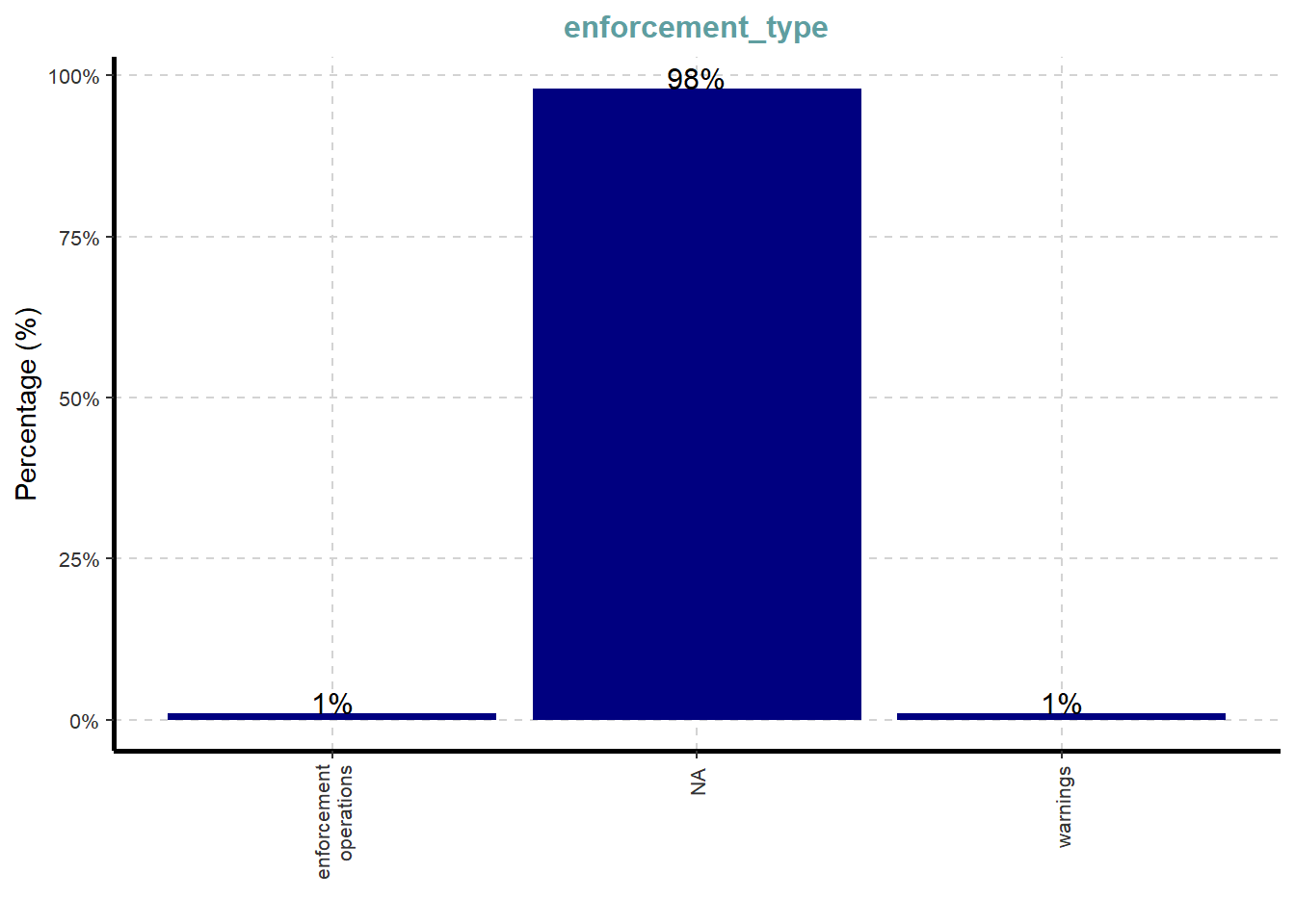
When there is an enforcement_type of enforcement operations or warnings, there might be an outcome at times.
When there is a movement_type, there might be a place of destination at times.
Observations of EDA from Relationship types:
When the subtype was coordinate, there were data in the field named coordination_types.
When the subtype was operate, there were data in the field named operational_roles.
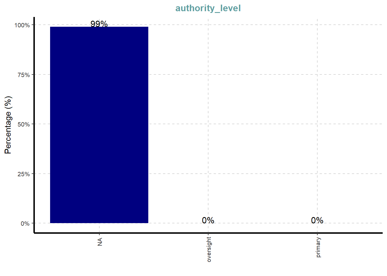
When there is a jurisdiction_type, there might be an authority_level.
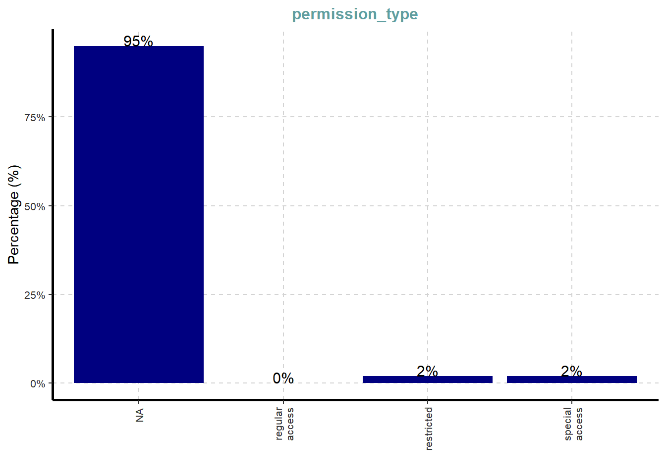
There are only restricted or special access data within permission_types.
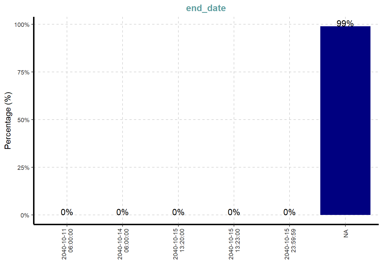
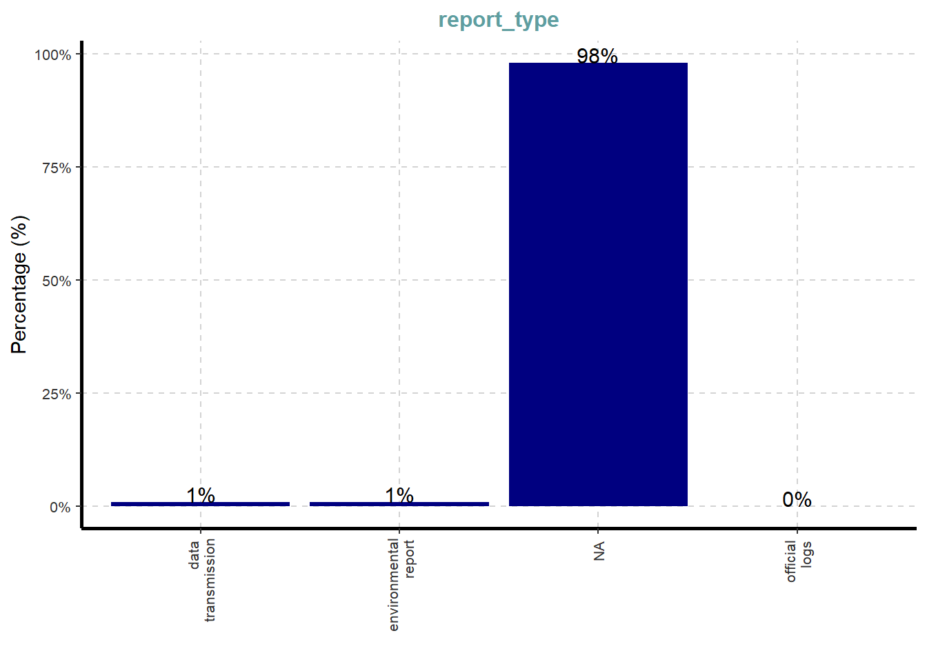
When there is a report_type of data transmission or environmental report, there might be a submission_date.
Observations of EDA from Entity types:
The 5 id under Group sub-types were not very useful information.
Elimination and directed focus:
Relative to the entire dataset, there were little assessment_type (3%), movement_type (2%), enforcement_type (2%), permission_type (4%), report_type (2%), authority_level (1%). We will direct our focus on other areas instead of these.
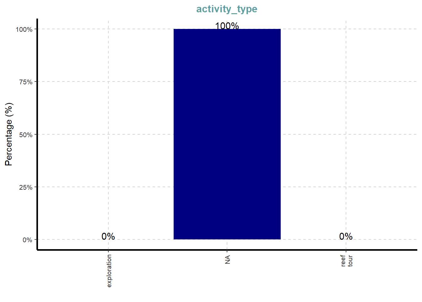
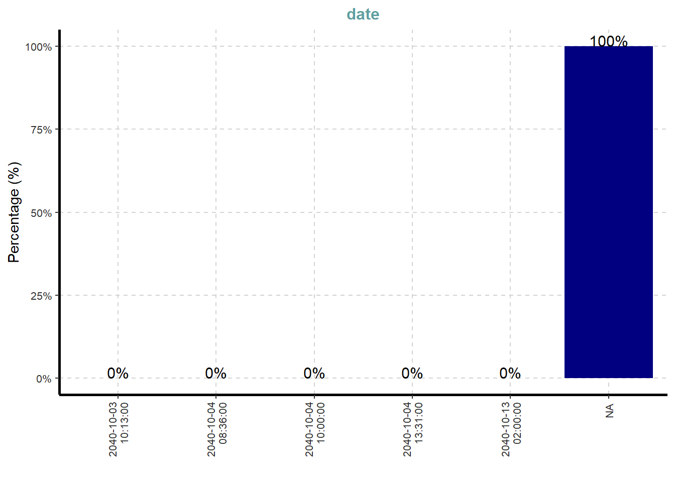
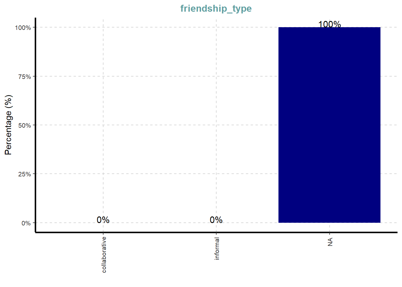
There were no to little useful data in the fields named: activity_type, references, dates, time, and friendship_type. These were not utilised.
We directed our focus on Event_Communication, Event_Monitoring, and Event_VesselMovement.
3.2 Edges
The code chunk below used ExpCATViz() of SmartEDA package to reveal the frequency distribution of all categorical fields in mc3_edges_raw tibble dataframe.
Entities are connected by edges to other Entities via an Event or Relationship node. The one exception to this is the Communication Event subtype, which is additionally linked to either an Event or Relationship node. The type field denotes the connector or edge type for the Entities, Event, and Relationship nodes. The edges are one of these: received, evidence_for, sent, NA.
Show the code
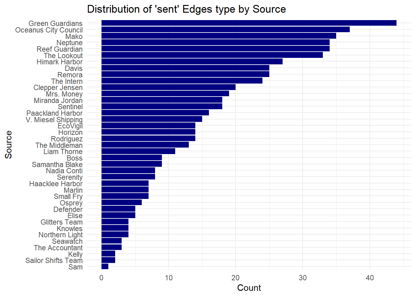
# Step 1: Filter for type == "sent"filtered_edges <- mc3_edges_raw %>%filter(type =="sent") %>%count(source) %>%arrange(desc(n)) %>%mutate(source =factor(source, levels =rev(unique(source)))) # descending # Step 2: Plotggplot(filtered_edges, aes(x = source, y = n)) +geom_col(fill ="navy") +coord_flip() +labs(title ="Distribution of 'sent' Edges type by Source",x ="Source",y ="Count" ) +theme_minimal()
What we understood from the information provided by Vast Challenge on Directional Edges:
For relationship as colleagues node or friends node, the node will have arrows/ edges pointing towards the relationship node.
For other relationships and events, the direction would be following the source and target.
renamed source and target fields to from_id and to_id respectively,
converted values in from_id and to_id fields to character data type,
excluded values in from_id and to_id which not found in the id field of mc3_nodes_cleaned,
excluded records whereby from_id and/or to_id values are missing, and
saved the cleaned tibble dataframe and called it mc3_edges_cleaned.
Show the code
mc3_edges_cleaned <- mc3_edges_raw %>%rename(from_id = source,to_id = target) %>%mutate(across(c(from_id, to_id), as.character)) %>%# Parse to_id to get supertype and sub_type for target nodes (e.g., Event_Communication)separate(to_id, into =c("to_id_supertype", "to_id_sub_type", "to_id_num"),sep ="_", remove =FALSE, fill ="right", extra ="merge") %>%# Filter to ensure from_id and to_id exist in mc3_nodes_cleaned (prevent orphaned edges)filter(from_id %in% mc3_nodes_cleaned$id, to_id %in% mc3_nodes_cleaned$id) %>%filter(!is.na(from_id), !is.na(to_id))print("Columns in mc3_edges_cleaned after initial cleaning:")
[1] "Columns in mc3_edges_cleaned after initial cleaning:"
print("Head of mc3_edges_cleaned after initial cleaning:")
[1] "Head of mc3_edges_cleaned after initial cleaning:"
Show the code
print(head(mc3_edges_cleaned))
# A tibble: 6 × 8
  id    is_inferred from_id to_id to_id_supertype to_id_sub_type to_id_num type
  <chr> <lgl>       <chr>   <chr> <chr>           <chr>          <chr>     <chr>
1 2     TRUE        Sam     Rela… Relationship    Suspicious     217       <NA>
2 3     FALSE       Sam     Even… Event           Communication  370       sent
3 5     TRUE        Sam     Even… Event           Assessment     600       <NA>
4 3013  TRUE        Sam     Rela… Relationship    Colleagues     430       <NA>
5 <NA>  TRUE        Sam     Rela… Relationship    Friends        272       <NA>
6 <NA>  TRUE        Sam     Rela… Relationship    Colleagues     215       <NA>
Show the code
# Find the number of unique types in each columnunique_counts <- mc3_edges_cleaned %>%summarise_all(n_distinct) %>%pivot_longer(cols =everything(), names_to ="column", values_to ="unique_count")# Print the unique counts for each columnprint(unique_counts)
Next, the code chunk below was used to join and convert from_id and to_id to integer indices. At the same time we also dropped rows with unmatched nodes.
Show the code
mc3_edges_indexed <- mc3_edges_cleaned %>%left_join(node_index_lookup, by =c("from_id"="id")) %>%rename(from = .row_id) %>%left_join(node_index_lookup, by =c("to_id"="id")) %>%rename(to = .row_id) %>%# Filter out edges where either source or target node was not foundfilter(!is.na(from) &!is.na(to)) %>%# Select all columns to carry forward to mc3_edges_finalselect(from, to, id, is_inferred, type, # Original edge attributes from_id, to_id, to_id_supertype, to_id_sub_type, to_id_num # Original IDs and parsed target type )
Next the code chunk below was used to subset nodes to only those referenced by edges.
Classes 'tbl_graph', 'igraph'  hidden list of 10
 $ : num 1159
 $ : logi TRUE
 $ : num [1:3226] 0 0 0 0 0 0 0 1 1 1 ...
 $ : num [1:3226] 1137 356 746 894 875 ...
 $ : NULL
 $ : NULL
 $ : NULL
 $ : NULL
 $ :List of 4
  ..$ : num [1:3] 1 0 1
  ..$ : Named list()
  ..$ :List of 28
  .. ..$ type             : chr [1:1159] "Entity" "Entity" "Entity" "Entity" ...
  .. ..$ label            : chr [1:1159] "Sam" "Kelly" "Nadia Conti" "Elise" ...
  .. ..$ name             : chr [1:1159] "Sam" "Kelly" "Nadia Conti" "Elise" ...
  .. ..$ sub_type         : chr [1:1159] "Person" "Person" "Person" "Person" ...
  .. ..$ id               : chr [1:1159] "Sam" "Kelly" "Nadia Conti" "Elise" ...
  .. ..$ timestamp        : chr [1:1159] NA NA NA NA ...
  .. ..$ monitoring_type  : chr [1:1159] NA NA NA NA ...
  .. ..$ findings         : chr [1:1159] NA NA NA NA ...
  .. ..$ content          : chr [1:1159] NA NA NA NA ...
  .. ..$ assessment_type  : chr [1:1159] NA NA NA NA ...
  .. ..$ results          : chr [1:1159] NA NA NA NA ...
  .. ..$ movement_type    : chr [1:1159] NA NA NA NA ...
  .. ..$ destination      : chr [1:1159] NA NA NA NA ...
  .. ..$ enforcement_type : chr [1:1159] NA NA NA NA ...
  .. ..$ outcome          : chr [1:1159] NA NA NA NA ...
  .. ..$ activity_type    : chr [1:1159] NA NA NA NA ...
  .. ..$ participants     : int [1:1159] NA NA NA NA NA NA NA NA NA NA ...
  .. ..$ reference        : chr [1:1159] NA NA NA NA ...
  .. ..$ permission_type  : chr [1:1159] NA NA NA NA ...
  .. ..$ start_date       : chr [1:1159] NA NA NA NA ...
  .. ..$ end_date         : chr [1:1159] NA NA NA NA ...
  .. ..$ report_type      : chr [1:1159] NA NA NA NA ...
  .. ..$ submission_date  : chr [1:1159] NA NA NA NA ...
  .. ..$ jurisdiction_type: chr [1:1159] NA NA NA NA ...
  .. ..$ authority_level  : chr [1:1159] NA NA NA NA ...
  .. ..$ coordination_type: chr [1:1159] NA NA NA NA ...
  .. ..$ operational_role : chr [1:1159] NA NA NA NA ...
  .. ..$ new_index        : int [1:1159] 1 2 3 4 5 6 7 8 9 10 ...
  ..$ :List of 8
  .. ..$ id             : chr [1:3226] "2" "3" "5" "3013" ...
  .. ..$ is_inferred    : logi [1:3226] TRUE FALSE TRUE TRUE TRUE TRUE ...
  .. ..$ type           : chr [1:3226] NA "sent" NA NA ...
  .. ..$ from_id        : chr [1:3226] "Sam" "Sam" "Sam" "Sam" ...
  .. ..$ to_id          : chr [1:3226] "Relationship_Suspicious_217" "Event_Communication_370" "Event_Assessment_600" "Relationship_Colleagues_430" ...
  .. ..$ to_id_supertype: chr [1:3226] "Relationship" "Event" "Event" "Relationship" ...
  .. ..$ to_id_sub_type : chr [1:3226] "Suspicious" "Communication" "Assessment" "Colleagues" ...
  .. ..$ to_id_num      : chr [1:3226] "217" "370" "600" "430" ...
 $ :<environment: 0x7fa52f667448>
 - attr(*, "active")= chr "nodes"
5.0 Knowledge Graphs
VisNetwork
VisNetwork provides the user to understand relationships through interactivity. For instance:
The individual nodes can be selected from the drop-down menu to view its connected nodes and edges.
The hover tooltip provides additional details from fields such as content, coordination_type, findings, destination, operational_role, results, and jurisdiction_type based on the related id information from mc3_nodes_final.
The Graph- VisNetwork
Show the code
# ---- 1. Define styles and legends ----event_subtypes <-c("Communication", "Monitoring", "VesselMovement", "Assessment","Collaborate", "Endorsement", "TourActivity", "TransponderPing","Harbor Report", "Fishing", "Criticize")relationship_subtypes <-c("Coordinates", "AccessPermission", "Operates", "Colleagues","Suspicious", "Reports", "Jurisdiction", "Unfriendly", "Friends")node_legend_colors_plot <-c("Person"="#88CCEE","Vessel"="#D55E00","Organization"="#117733","Location"="#AA4499","Group"="#CC79A7","Event"="#DDCC77", # type level"Relationship"="#AF8DC3"# type level)node_legend_shapes_plot <-c("Person"="dot","Vessel"="triangle","Organization"="square","Location"="diamond","Group"="circle plus","Event"="star", # type level"Relationship"="square x"# type level)STYLES <-list(node_label_dark ="black",font_family ="Roboto Condensed")# ---- 2. Prepare nodes ----nodes <- mc3_nodes_final %>%mutate(label =ifelse(is.na(name), id, name),# These parts are for pulling the related data from other fieldstooltip_extra =case_when( type =="Event"& sub_type =="Communication"~ content, type =="Event"& sub_type =="Monitoring"~ findings, type =="Event"& sub_type =="VesselMovement"~ destination, type =="Event"& sub_type =="Assessment"~ results, type =="Relationship"& sub_type =="Coordinates"~ coordination_type, type =="Relationship"& sub_type =="Operates"~ operational_role, type =="Relationship"& sub_type =="Jurisdiction"~ jurisdiction_type,TRUE~NA_character_ ),title =paste0("<b>", label, "</b><br>","Type: ", type, "<br>","Sub-type: ", sub_type, "<br>",ifelse(!is.na(tooltip_extra), paste0("<br><b>Details:</b> ", tooltip_extra), "") ),# Fallback logic: if sub_type is NA or not in styling list, use type insteadgroup =ifelse(sub_type %in%names(node_legend_colors_plot), sub_type, type) ) %>%select(id, label, group, title) %>%distinct()# ---- 3. Prepare directed edges (type == "sent") ----edges <- mc3_edges_final %>%filter(from_id %in% nodes$id & to_id %in% nodes$id) %>%select(from = from_id, to = to_id)# ---- 4. Build visNetwork ----net <-visNetwork(nodes, edges, width ="100%", height ="600px") %>%visEdges(arrows =list(to =list(enabled =TRUE, scaleFactor =1.5))) %>%visOptions(highlightNearest =TRUE, nodesIdSelection =TRUE) %>%visIgraphLayout(layout ="layout_with_fr") %>%visNodes(font =list(size =14,color = STYLES$node_label_dark,face = STYLES$font_family,vadjust =-15 ))# ---- 5. Apply shape and color per group ----for (group_name innames(node_legend_colors_plot)) { net <- net %>%visGroups(groupname = group_name,color = node_legend_colors_plot[[group_name]],shape = node_legend_shapes_plot[[group_name]] )}# ---- 6. Add legend ----used_groups <-unique(nodes$group)legend_df <- tibble::tibble(label = used_groups,shape = node_legend_shapes_plot[used_groups],color = node_legend_colors_plot[used_groups]) %>%distinct(label, .keep_all =TRUE) # remove duplicates just in casenet <- net %>%visLegend(addNodes = legend_df,ncol =2, # number of columnsposition ="left", main ="Entity (Sub)Types", # titleuseGroups =FALSE# show custom legend entries)# ---- 7. Render ----net
# Split the 'from_id' columnmc3_edges_cleaned <- mc3_edges_cleaned %>%separate(from_id, into =c("from_id_supertype", "from_id_sub_type", "from_id_id"), sep ="_", remove =FALSE, extra ="drop")# Split the 'target' column into mc3_edges_cleaned <- mc3_edges_cleaned %>%separate(to_id, into =c("to_id_supertype", "to_id_sub_type","to_id_id"), sep ="_", remove =FALSE, extra ="drop")# Find the number of unique types in each columnunique_counts <- mc3_edges_cleaned %>%summarise_all(n_distinct) %>%pivot_longer(cols =everything(), names_to ="column", values_to ="unique_count")# Print the unique counts for each columnprint(unique_counts)
# Check the mappingmc3_edges_cleaned %>%group_by(from_id_supertype, from_id_sub_type) %>%summarize(count =n()) %>%arrange(-count) %>%kable()
from_id_supertype
from_id_sub_type
count
Event
Communication
1620
Green Guardians
NA
90
Relationship
Coordinates
81
Mako
NA
78
Reef Guardian
NA
72
Relationship
AccessPermission
63
Oceanus City Council
NA
62
Remora
NA
62
Event
Monitoring
59
Neptune
NA
57
EcoVigil
NA
51
Sentinel
NA
47
Davis
NA
46
The Lookout
NA
44
Event
VesselMovement
43
Relationship
Operates
41
The Intern
NA
37
Event
Assessment
33
Horizon
NA
32
V. Miesel Shipping
NA
32
Himark Harbor
NA
31
Mrs. Money
NA
31
Miranda Jordan
NA
30
Clepper Jensen
NA
27
Liam Thorne
NA
26
Relationship
Suspicious
26
Relationship
Reports
25
Rodriguez
NA
25
Event
Enforcement
23
Paackland Harbor
NA
22
Boss
NA
21
The Middleman
NA
19
Event
Collaborate
17
Nadia Conti
NA
17
Small Fry
NA
17
Marlin
NA
15
Osprey
NA
15
Samantha Blake
NA
15
Serenity
NA
15
Event
TourActivity
14
Relationship
Jurisdiction
14
Defender
NA
12
Knowles
NA
12
Seawatch
NA
12
Elise
NA
10
Glitters Team
NA
9
Haacklee Harbor
NA
9
Sailor Shifts Team
NA
9
Northern Light
NA
8
The Accountant
NA
8
Sam
NA
7
Relationship
Unfriendly
5
Conservation Vessels
NA
4
Kelly
NA
4
Event
HarborReport
3
Event
TransponderPing
3
Mariner’s Dream
NA
3
Recreational Fishing Boats
NA
3
Port Security
NA
2
Relationship
Colleagues
2
Tourists
NA
2
Diving Tour Operators
NA
1
Event
Criticize
1
Event
Fishing
1
Sailor Shift
NA
1
Show the code
# Check the mappingmc3_edges_cleaned %>%group_by(to_id_supertype, to_id_sub_type) %>%summarize(count =n()) %>%arrange(-count) %>%kable()
to_id_supertype
to_id_sub_type
count
Event
Communication
584
Event
Monitoring
240
Relationship
AccessPermission
225
Relationship
Coordinates
207
Event
VesselMovement
160
Relationship
Colleagues
160
Relationship
Operates
129
Event
Assessment
103
Nemo Reef
NA
102
Mako
NA
89
Relationship
Reports
72
Oceanus City Council
NA
68
Relationship
Suspicious
68
Relationship
Jurisdiction
63
Event
Collaborate
62
Remora
NA
60
Event
Enforcement
47
Neptune
NA
45
Himark Harbor
NA
38
Reef Guardian
NA
38
Green Guardians
NA
37
Sentinel
NA
36
V. Miesel Shipping
NA
35
Event
TourActivity
32
Horizon
NA
32
Paackland Harbor
NA
29
Mrs. Money
NA
26
Boss
NA
24
EcoVigil
NA
21
Miranda Jordan
NA
20
Nadia Conti
NA
20
Protected areas
NA
20
Clepper Jensen
NA
19
Davis
NA
18
The Intern
NA
18
Liam Thorne
NA
17
Seawatch
NA
16
Event
TransponderPing
12
Sailor Shifts Team
NA
12
Relationship
Unfriendly
11
Serenity
NA
11
Marlin
NA
10
Restricted Zone
NA
10
Sam
NA
10
Restricted areas
NA
9
Rodriguez
NA
9
South Dock
NA
9
The Lookout
NA
9
Haacklee Harbor
NA
7
Samantha Blake
NA
7
The Middleman
NA
7
Eastern reefs
NA
6
Elise
NA
6
Knowles
NA
6
Northern quadrant
NA
6
Relationship
Friends
6
Western quadrant
NA
6
Dolphin Bay
NA
5
Eastern Boundary
NA
5
Northern Light
NA
5
Western Boundary
NA
5
Eastern quadrant
NA
4
City Officials
NA
3
Coral Point
NA
3
Defender
NA
3
E7
NA
3
Event
HarborReport
3
Osprey
NA
3
Route C
NA
3
The Accountant
NA
3
Berth 14
NA
2
Castaway Cove
NA
2
Eastern Islands
NA
2
Eastern Shoals
NA
2
Event
Criticize
2
Event
Fishing
2
Mariner’s Dream
NA
2
Southern Boundary
NA
2
Southern coastline
NA
2
Southern islands
NA
2
Azure Cove
NA
1
Conservation Vessels
NA
1
Eastern Coastline
NA
1
Glitters Team
NA
1
Kelly
NA
1
Port Security
NA
1
Recreational Fishing Boats
NA
1
Small Fry
NA
1
Southern quadrant
NA
1
Under Event-Communication types: The edges target type and target subtypes matches the count of 584 for node to_id_supertype and node to_id_sub_type. However, there were only 581 count for content within the original node file. We then looked into duplicates.
# A tibble: 5 × 2
  content                                                                      n
  <chr>                                                                    <int>
1 Boss, The Accountant here. Conservation vessels deploying underwater mi…     2
2 Davis here to V. Miesel Shipping. Crew reallocation from Remora to Nept…     2
3 Mrs. Money, this is Middleman. I've redirected Council's attention to o…     2
4 Rodriguez, Davis here. Maintain current position with Mako at Nemo Reef…     2
5 <NA>                                                                       575
There were 4 duplicates within the content column. Upon checking the original data, one was the sender and the other was the receiver who received the same content. We left the data as it was.